As a business location, Germany has been suffering from deteriorating competitiveness for some years now. This is due to price factors and non-price factors and is reflected in a loss of export market share. While previous Bundesbank analyses have used granular trade data to decompose German export market share losses into demand-side and supply-side components and interpreted the latter in the sense of a broadly understood, revealed competitiveness, the present analysis focuses on macroeconomic indicators of price competitiveness. The results are therefore complementary: Germany’s price competitiveness has deteriorated markedly over the past decade. At the same time, German exports have lost momentum and have been declining since 2022. This article examines how closely these two developments are related. To this end, it draws on Bundesbank indicators of price competitiveness and uses a dataset of more than 50 countries to analyse their impact on export developments from 1980 onwards.

The results show that a deterioration in price competitiveness generally has a measurable dampening effect on export growth. At the same time, however, price competitiveness indicators explain only a limited part of the recent weakness in German exports. Depending on the indicator, the deterioration in price competitiveness as of 2022 explains between 6 % and 24 % of the deviation of average export growth in the 2022‑25 period from the pre-pandemic trend growth in the 2015‑19 period. The highest explanatory contribution is thus around one-quarter. In addition, weaker demand from trading partners for imports can also explain up to around one-quarter of the deviation from the pre-pandemic export trend.

The analysis thus supports the findings of previous studies showing that Germany’s recent weakness in exports is not solely attributable to price factors or cyclical headwinds. Instead, structural factors are also likely to have played a role. These include sectoral cost burdens, which macroeconomic indicators only partially capture, as well as the product mix of German exports and business conditions in Germany. This is in line with previous Bundesbank analyses, which point to sectoral losses in competitiveness and supply-side burdens on Germany’s export industry. Overall, the results underscore the need for a broad-based strengthening of Germany’s competitiveness.

1 Introduction

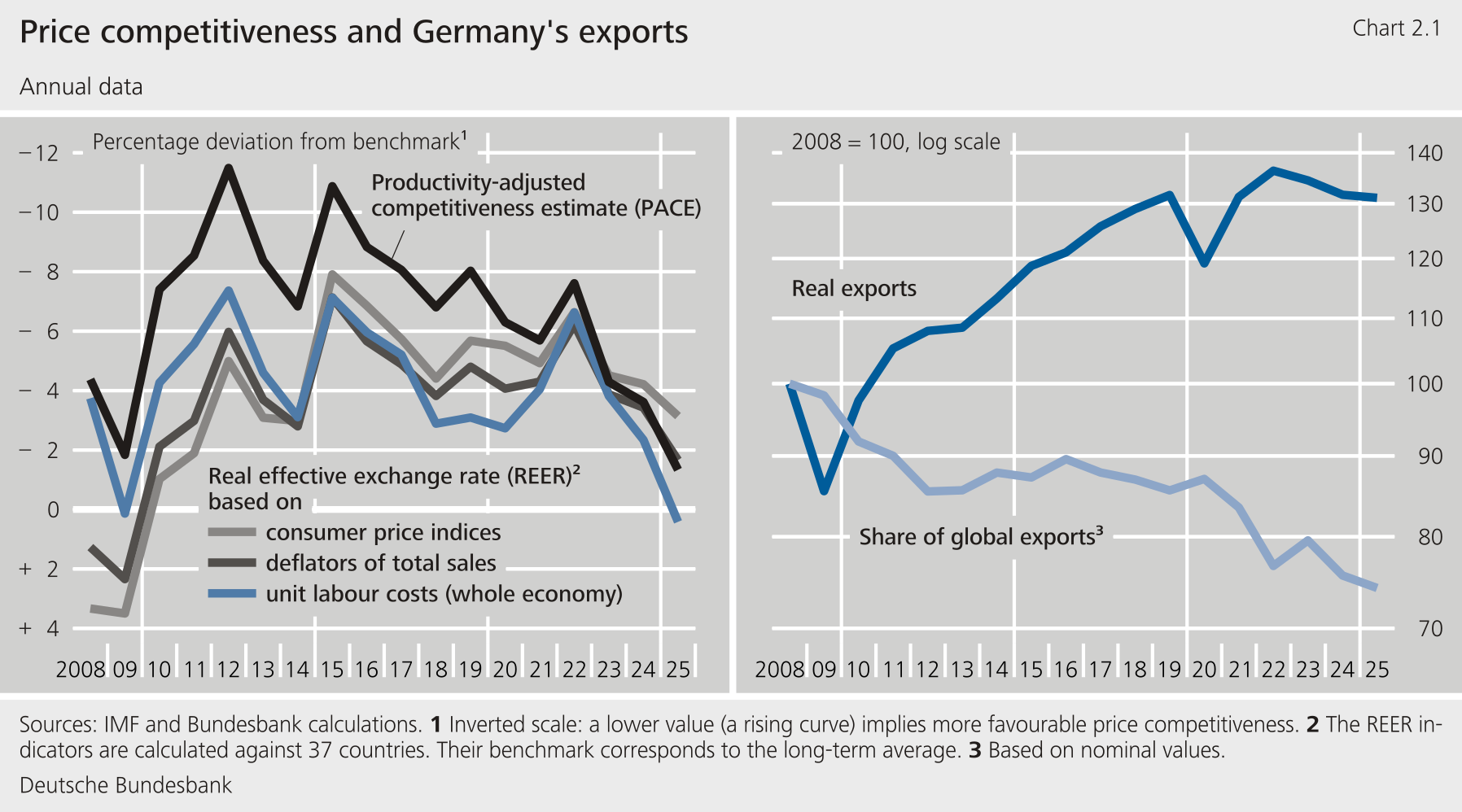
Germany has been losing price competitiveness for around a decade. The left-hand side of Chart 2.1 illustrates changes in price competitiveness based on several indicators. As well as showing various real effective exchange rates (REERs), it also displays the “productivity‑adjusted competitiveness estimate” (PACE), an indicator developed at the Bundesbank. 1 The real effective exchange rate measures a country’s relative price level in aggregate terms relative to its trading partners, for example on the basis of consumer prices, unit labour costs, or the deflator of total sales. 2 An appreciation of the real effective exchange rate worsens the price competitiveness of the country under review. However, focusing solely on price level differences may be too simplistic. The PACE indicator therefore goes beyond the mere analysis of prices to cover productivity differences, as under otherwise identical circumstances, higher productivity is associated with more favourable competitiveness. 3 Put simply, the PACE indicator thus shows the relative price level that can still be considered neutral for a country in light of its productivity, on the one hand, and that of its competitors in its sales markets, on the other. If the actual price level is higher than this, price competitiveness is unfavourable. The indicators paint a consistent picture of developments: Germany’s price competitiveness has been on a downward trend for around ten years that has recently become even more unfavourable than before.

At the same time, Germany’s export growth has slowed in recent years and has actually been negative since 2022. The darker curve on the right-hand side of Chart 2.1 shows Germany’s real exports as of 2008. Following a sharp rise in the 2010s, exports plummeted in 2020 due to the pandemic but subsequently recovered just as quickly. Real exports declined between 2022 and 2025. However, German export growth had already fallen behind that of its trading partners before this point in time. Accordingly, Germany’s share in the global export market declined continuously as of 2017. 4

Price competitiveness and Germany's exports

This article examines the extent to which this weak development in German exports can be explained by the observed deterioration in price competitiveness. An important quality criterion for indicators of price competitiveness is their ability to help explain observed export patterns. However, there is no mechanical 1:1 relationship between changes in price competitiveness and export growth. Countries with diminished price competitiveness can still achieve high export growth. This is because, in addition to price competitiveness, numerous other factors influence exports, such as their product mix, demand from trading partners or structural business conditions. Nevertheless, a statistical relationship between changes in price competitiveness and export growth should be verifiable in a broad comparison of countries over the long term. The study presented below therefore uses a dataset of more than 50 countries going back to 1980 to estimate the relationship between price competitiveness and export growth. In order to assess German export developments as of 2022, a two-step approach is taken. First, the international dataset is used to calculate response coefficients that are uniform across countries and which indicate how strongly export growth responds on average to changes in price competitiveness across the entire sample. For Germany, a hypothetical export trajectory is then determined using the coefficients calculated in this way. This shows how Germany’s real exports would have developed if the country’s price competitiveness had not deteriorated any further as of 2022.

2 Price competitiveness and exports in an international comparison

The analysis uses annual time series of price competitiveness and export data for over 50 countries from 1980 onwards. The indicators of price competitiveness used include the aforementioned real effective exchange rates, which are calculated on the basis of either the consumer price index, the deflator of total sales, or unit labour costs in the economy as a whole. 5 The estimation takes into account these REER indicators for 38 countries. They are expressed relative to the long-term average of the respective time series to enable comparisons across countries. 6 In addition to the REER indicators, the PACE indicator, which is also described above, is used as well. Estimations using this indicator take into account a larger sample of 57 countries. 7 Price-adjusted exports of goods and services are used as the export variable. 8

A panel regression with distributed lags is used to estimate how changes in price competitiveness affect export growth. The analysis uses foreign demand and lagged domestic economic activity, as well as country and annual effects as control variables. The supplementary information entitled “How is the relationship between price competitiveness and exports estimated?” explains the methodological details of the estimation specification. It also presents a supplementary specification in levels that allows assessments to be made about long-term relationships between price competitiveness and export levels.

Supplementary information

How is the relationship between price competitiveness and exports estimated?

A panel model is used to estimate how changes in price competitiveness affect export growth. The dependent variable is real export growth. The respective indicator of price competitiveness is included as an explanatory variable with up to two lags to capture both short-term and lagged responses of export growth. It is estimated using annual data. The complete estimation equation takes the form

$$ \begin{align} \Delta\ln X_{i,t} &= \alpha_i + \tau_t + \beta_0 \Delta z_{i,t} +\beta_1\Delta z_{i,t-1} + \beta_2 \Delta z_{i,t-2} \\&+ \gamma_0 \Delta \ln FD_{i,t} +\gamma_1 \Delta \ln FD_{i,t-1} +\theta \Delta \ln Y_{i,t-1} +\varepsilon_{i,t} \end{align} $$

Here, $ X_{i,t} $ denotes real exports of country $ i $ in year $ t $. The variable $ z_{i,t} $ represents the respective indicator of price competitiveness: the logarithmic indicator is used for real effective exchange rates; for the PACE indicator, however, the deviation from the benchmark is measured in percentage points. $ FD_{i,t} $ measures foreign demand as the trade-weighted sum of partner countries’ GDP. 1 $ Y_{i,t} $ denotes domestic GDP. The terms $ \alpha_i $ and $ \tau_t $ represent country and time fixed effects.

An increase in the variable $ z $ corresponds to a deterioration in price competitiveness. For the REER indicators, this is a real effective appreciation; for the PACE indicator, weak domestic productivity developments relative to other countries can also contribute to the increase of $ z $. The coefficient therefore measures the immediate impact of such a deterioration on export growth in the same year. The sum $ \beta_0 +\beta_1+\beta_2$ approximates the extent to which real export growth changes after two more years if there is an initial and lasting deterioration in price competitiveness of 1 % or of 1 percentage point in the case of the PACE indicator. 2 Accordingly, $ \gamma_0 + \gamma_1 $ measures the cumulative effect of a change in foreign demand on export growth after the subsequent year.

Control variables and fixed effects help to isolate the relationship between price competitiveness and exports. The country fixed effects capture time-invariant differences between countries. The annual fixed effects control for global shocks that impact all countries simultaneously. Such shocks occurred, for example, in 2008‑09 during the financial crisis and in 2020‑21 during the pandemic. Foreign demand is taken into account because exports can rise even when price competitiveness remains unchanged if demand from trading partners grows. Lagged domestic GDP growth controls for domestic factors, such as investment, which can also have a positive effect on exports. It is only entered with a lag, given that higher exports in the same year can also increase domestic GDP and the lag thus avoids an endogeneity problem.

Potential endogeneity problems should also be kept in mind with regard to the variable of interest: price competitiveness. This is necessary because the competitiveness indicator and exports may have a reciprocal effect on each other. For instance, rising exports can contribute to an appreciation of the domestic currency or push up margins and export prices and thus, in turn, have an impact on price competitiveness indicators. In addition, common shocks, such as energy price shocks, can simultaneously affect exchange rates, prices and exports. The control variables and fixed effects help to contain this endogeneity problem.

The specification assumes uniform price elasticities for all countries. The assumption of uniform values for all countries for $ \beta_0 $, $ \beta_1 $ and $ \beta_2 $ is restrictive, as countries differ in terms of their export structure, exchange rate regime, import dependency, the importance of global value chains and sectoral specialisation, for example. However, compared with a pure time series analysis, the panel analysis has the advantage for Germany that it is able to use significantly more variation cross-sectionally and longitudinally. A time series analysis for Germany would be based on relatively few annual observations and could be strongly influenced by individual episodes such as the financial crisis, the pandemic or the surge in energy prices. In the panel, however, country and annual fixed effects can be taken into account, meaning that the estimation is adjusted for permanent country differences and global shocks. The estimated coefficients of price competitiveness should be interpreted as average responses of exports in the panel.

For all indicators, the estimated coefficients indicate a negative relationship between a deterioration in price competitiveness and export growth. Table 2.1 shows the estimation results including standard errors. In the baseline specification, the standard errors are clustered at country level. The results remain robust if the standard errors are calculated instead using country and year clustering or according to Driscoll and Kraay (1998). In both cases, the significance of the competitiveness coefficients is retained.

**Table 2.1: Regression results of the baseline specification**
Indicator	$ \beta_0 $	$ \beta_0 + \beta_1 + \beta_2 $	$ \gamma_0 $	$ \theta $	R²	N	Number of countries
PACE	– 0.168 (0.038; p < 0.001)	– 0.235 (0.043; p < 0.001)	0.311 (0.140; p = 0.027)	0.246 (0.098; p = 0.012)	0.491	1 549	57
REER consumer prices	– 0.122 (0.031; p < 0.001)	– 0.232 (0.081; p = 0.004)	0.477 (0.165; p = 0.004)	0.184 (0.121; p = 0.128)	0.537	1 073	38
REER total sales deflator	– 0.177 (0.047; p < 0.001)	– 0.295 (0.075; p < 0.001)	0.513 (0.235; p = 0.029)	0.139 (0.105; p = 0.184)	0.550	918	38
REER unit labour costs	– 0.251 (0.056; p < 0.001)	– 0.382 (0.106; p < 0.001)	0.453 (0.193; p = 0.019)	0.238 (0.129; p = 0.064)	0.564	952	38
Notes: standard error and p-value in brackets; baseline specification with standard errors clustered at country level. N = number of observations. γ₁ is largely insignificant and is therefore not shown.

In addition, the relationship is estimated with level data in order to determine long-term coefficients. As an alternative to estimating in rates of change, the following specification is estimated in levels:

$$ \begin {align*} \ln X_{i,t} = \alpha_i + \tau_t + \beta^L z_{i,t} + \gamma^L \ln FD_{i,t} + \theta^L \ln Y_ {i,t-1} + u_{i,t}. \end {align*} $$

Given that the variables are entered in logarithmic levels, the coefficient $ \beta^L $ can be understood as long-term elasticity. It measures the percentage by which the export level changes if there is a lasting change in the competitiveness indicator of 1 % or of 1 percentage point in the case of the PACE indicator.

Footnotes

For a given base country, all other countries in the sample are deemed partner countries. GDP data are taken from the IMF’s WEO database and expressed in constant US dollars. In the baseline specification, foreign demand is calculated as the partner countries’ trade-weighted GDP. Alternatively, foreign demand is calculated on the basis of the partner countries’ trade-weighted imports. These are also weighted because not all foreign import demand is equally relevant for the base country’s exports: sales markets that the country is more focused on are given a higher weight. This alternative specification hardly changes the estimated role of price competitiveness, but it increases the contribution of foreign demand to explaining export developments.
A change in the competitiveness indicator influences export growth in the estimation in the current year as well as with a one and two-year lag. Since the export level corresponds to the cumulative growth in exports, the change in the logarithmic export level compared with a hypothetical path with constant price competitiveness is derived from the sum of these estimated contributions to growth. For small changes, this log change can be approximated as a percentage change in the export level.

Impact of a deterioration in price competitiveness on real exports

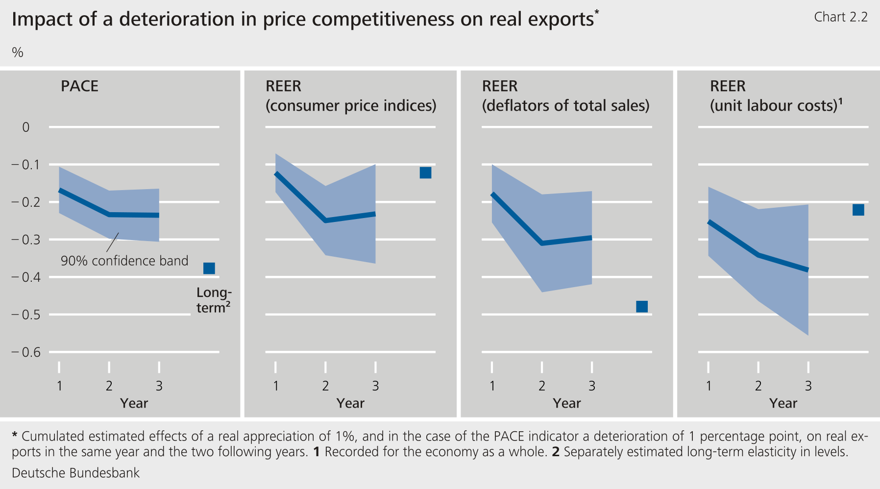
If price competitiveness deteriorates, real export growth slows significantly over the course of three years, with significant effects already occurring in the short term. For the various indicators of price competitiveness, Chart 2.2 shows how real export growth declines if competitiveness deteriorates. A real effective appreciation of 1 % (or in the case of the PACE indicator a deterioration in price competitiveness of 1 percentage point) is assumed, which begins in the first year and is permanent. The picture is uniform across the various measures: if all the other factors remain unchanged, such a deterioration in price competitiveness is accompanied by lower export growth rates. The negative effect already emerges in the same year and increases cumulatively over the subsequent one to two years. Depending on the indicator, the cumulative response to a reduction in real exports after three years is around 0.2 % to 0.4 %. The estimated effects differ only to a limited extent between the indicators. The response is strongest for the real effective exchange rate based on unit labour costs, and weakest for the consumer price-based measure. The additionally presented long-term estimates suggest that a permanent deterioration in price competitiveness can weigh on exports somewhat more strongly than the cumulative effects over three years indicate. However, this is not the case for all indicators. The relationship is weaker and less robust in the long term for the real effective exchange rate based on consumer prices and for the indicator based on unit labour costs. 9 The export price elasticities estimated here are in line with the results of the relevant literature. 10

Supplementary information

Can indicators of price competitiveness explain differences in export levels in an international comparison?

In addition to the question of whether they explain export growth, it is also of interest whether indicators of price competitiveness contribute to determining the export level in a cross-country comparison. The analysis presented above showed that developments in a country’s exports over time can be explained by developments in price competitiveness: if price competitiveness improves, this typically goes hand in hand with stronger export growth. However, for an economic assessment, a cross-country comparison is also of interest. This raises the question of whether a country with more favourable price competitiveness also has a higher export level on average than a country with less favourable price competitiveness. An indicator can only provide an answer to this if it is capable of systematically explaining differences between the export levels of different countries. This supplementary information explores this question. To this end, export levels are made comparable across countries by normalising them using the corresponding GDP figure. The export ratio is therefore examined below.

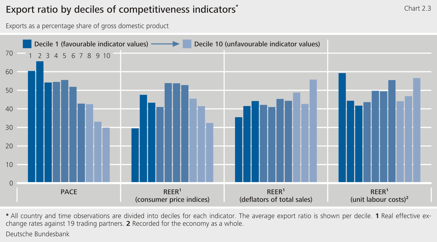
A graphical analysis shows that observations with more favourable PACE values are associated with higher export ratios; REER-based indicators do not show such a relationship. An initial approach to the question is provided by a graphical evaluation. To this end, the values of the respective indicator of price competitiveness for all countries and points in time are considered together and sorted according to their size – from particularly favourable to particularly unfavourable competitive positions. The sorted values of the indicator under consideration are then divided into ten groups (deciles). Chart 2.3 shows the average export ratio for each of these deciles. The PACE indicator shows a clear relationship: observations with favourable price competitiveness are associated with higher export ratios on average. As the competitive position deteriorates, the export ratio declines across the deciles. By contrast, a similar pattern does not exist for real effective exchange rates. Export ratios fluctuate across the deciles without any discernible systematic relationship. This suggests that these indicators are barely able to capture differences between countries’ export levels.

Export ratio by deciles of competitiveness indicators

An econometric analysis confirms the result shown in the chart: only the PACE indicator is able to make a significant contribution to determining export ratios. In a statistical estimate, only the PACE indicator explains the export ratio to a statistically significant extent. 1 Specifically, according to the PACE indicator, price competitiveness that is less favourable by 1 percentage point is associated with a reduction in the export ratio of around 0.4 percentage point. By contrast, there is no statistically significant relationship between real effective exchange rates and the export level. Overall, the results thus suggest that the level data contained in the PACE indicator (relative price and productivity level) help better gauge the international competitiveness of economies, a quality that index-based indicators lack. While real effective exchange rates mainly capture changes in competitiveness over time, the PACE indicator is also suitable for explaining differences between export levels across countries. 2

Footnotes

This is estimated in a pooled dataset $ \ln (X_{i,t} / GDP_{i,t}) = \alpha + \beta_Z \ln Z_{i,t} + \gamma \ln FD_{i,t} + \tau_t + \varepsilon_{i,t} $, where $ X_{i,t} / GDP_{i,t} $ denotes the export ratio and $ FD_{i,t} $ the weighted GDP of the trading partners. The term $ Z $ refers to the indicator of price competitiveness used, and $ \tau $ are annual fixed effects. Country fixed effects are deliberately not included to prevent them filtering out differences in levels. Unlike real effective exchange rates, the PACE indicator is not logarithmic because it is defined as a percentage deviation from the benchmark.
However, these considerations do not play a direct role in the scenario analysis of German exports described below, as this analysis exclusively considers changes in competitiveness over time.

3 How much of a drag on Germany’s exports has been caused by the deterioration in price competitiveness?

Using hypothetical scenarios, it is possible to estimate how much the deterioration in price competitiveness as of 2022 has dampened developments in German exports. As mentioned at the outset, there have been unfavourable developments in both Germany’s price competitiveness and its exports in recent years, especially as of 2022. The results of the previous section show that a deterioration in price competitiveness has a statistically significant impact on export growth. This raises the question of the extent to which Germany’s recent weakness in exports can actually be attributed to the deterioration in price competitiveness. This can be estimated using a “counterfactual analysis”, comparing actual export developments with a hypothetical path that would have occurred if price competitiveness had not continued to deteriorate as of 2022. By contrast, other factors – such as foreign demand or domestic growth – are assumed to have developed as actually observed. This allows us to estimate how much the deterioration in price competitiveness as of 2022 alone weighed on exports.

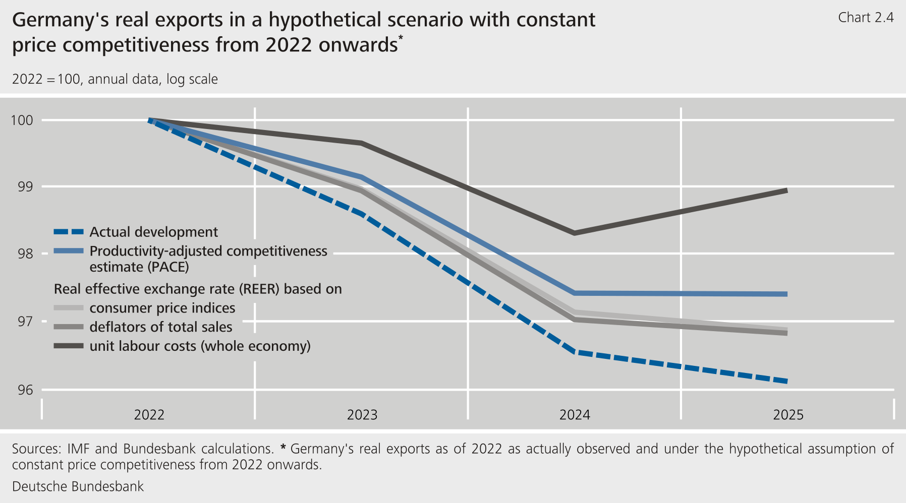
The analysis suggests that the deterioration in price competitiveness as of 2022 weighed markedly on German exports but only accounts for a limited part of the recent weakness in exports. Chart 2.4 illustrates the first of these two statements for the various indicators of price competitiveness. It shows actually observed developments in Germany’s real exports as of 2022 as well as hypothetical developments that would have arisen if the respective price competitiveness had not deteriorated further from that point onwards. In all cases, exports calculated for the hypothetical scenario are higher than those actually observed. This indicates that the deterioration in price competitiveness has indeed weighed on German exports in recent years. The extent of this burden is shown by a comparison with export growth prior to the coronavirus pandemic. Between 2015 and 2019, Germany’s real exports grew by an average of 2.6 % per year. 11 By contrast, growth declined as of 2022, with exports contracting by an average of 1.3 % per year in the 2022‑25 period. If price competitiveness had not continued to deteriorate as of 2022, export developments would not have been as weak. In this case, real exports would have declined by just under 0.3 % per year in the most favourable case, depending on the indicator. Measured in terms of the overall difference to the pre-pandemic growth trend (just under 4 percentage points), only around one-quarter of the weaker export growth (1 percentage point) can therefore be explained by the price factors examined here. 12 However, the actual weaker foreign demand also narrows the gap to the pre-pandemic trend. Depending on the specification, it explains a maximum of 0.9 percentage point of the decline in the export growth rate and thus around 22 % to 23 % of the gap to the pre-pandemic trend. 13

Germany's real exports in a hypothetical scenario with constant price competitiveness from 2022 onwards

In terms of their impact on German export developments, these indicators show differences in degree but share the same basic assessment. The strongest effect is provided by the real effective exchange rate based on unit labour costs in the economy as a whole. This is partly because this indicator had the highest estimated export price elasticity. In addition, Germany’s price competitiveness as measured by this indicator deteriorated particularly significantly as of 2022. The results for the other indicators also suggest that exports would have developed somewhat more favourably if price competitiveness had remained unchanged. However, the respective gap to actual export developments is smaller.

As the price factors considered here explain Germany’s export weakness only to a limited extent, the question arises as to which other factors could have played a role. Previous Bundesbank analyses show that supply-side factors explain a major part of the German export industry’s losses in market share. These may also include cost factors that are only partially captured by the aggregate macroeconomic indicators of price competitiveness. These factors are probably particularly relevant due to the pronounced heterogeneity of Germany’s export industry. For example, a macroeconomic indicator can mask the fact that individual export-based sectors were exposed to significantly stronger cost surges than others. This applies, for example, to energy-intensive sectors, for which the sharp rise in energy prices in Germany compared to other countries is likely to have particularly weighed on price competitiveness. In these sectors, price burdens may therefore have contributed more to weak export developments than macroeconomic indicators would suggest. In addition, domestic business conditions are likely to have weighed on export developments. Furthermore, previous analyses show that the specific product mix of Germany’s export industry has dampened export market shares in recent years. Germany specialises particularly strongly in categories of goods for which global demand was weak.

4 Conclusion

The Bundesbank’s indicators show that price competitiveness has a statistically significant impact on exports. The analysis presented here shows for a large number of countries that both changes in real effective exchange rates based on various deflators and changes in the Bundesbank’s PACE indicator explain export growth to a statistically significant extent. According to this analysis, export growth declines by a cumulative 0.2 % to 0.4 % per 1 % real appreciation. In contrast to real effective exchange rates, the PACE indicator can also explain why some countries have high export ratios and others have lower export ratios. 14

Although Germany’s markedly lower price competitiveness in recent years has contributed to the country’s current export weakness, it can only explain a limited part of it. A comparison with hypothetical scenarios suggests this. According to the present analysis, and depending on the indicator used, a maximum of one-quarter of the weaker export developments in 2022‑25 compared with the pre-pandemic trend growth can be ascribed to deteriorating price competitiveness. Weaker foreign demand explains a maximum of another one-quarter of the deviation in export developments. Factors beyond this, such as the structure of German sales markets and of the range of German exports, or cost burdens that are only relevant for key sectors, are therefore likely to account for a marked share of the weakness in exports.

Against this backdrop, a broad-based approach to strengthening Germany’s international competitiveness appears necessary. This includes measures that have a direct impact on enterprises’ costs, such as non-wage labour costs, and which are thus reflected in the indicators used here. However, given the additional burdens, it is also important to improve structural business conditions that strengthen the productivity of Germany’s export industry, as well as its ability to innovate and adapt. These include a reliable framework for private investment, better conditions for research and development, better conditions for young, innovative enterprises, faster digitalisation and, in particular, lower costs of bureaucracy. 15

List of references

Ahmed, S., M. Appendino and M. Ruta (2017), Global value chains and the exchange rate elasticity of exports, The BE Journal of Macroeconomics, Vol. 17(1), 2015‑0130.

Bems, R. and R. C. Johnson (2017), Demand for Value Added and Value-Added Exchange Rates, American Economic Journal: Macroeconomics, Vol. 9(4), pp. 45‑90.

Bussière, M., G. Gaulier and W. Steingress (2020), Global trade flows: Revisiting the exchange rate elasticities, Open Economies Review, Vol. 31(1), pp. 25‑78.

Deutsche Bundesbank (2026a), Latest developments in German export market shares and their driving forces, Monthly Report, March 2026.

Deutsche Bundesbank (2026b), Statistical Series – Exchange rate statistics.

Deutsche Bundesbank (2026c), Cause and effect of growing bureaucratic burdens in Germany’s corporate sector, Monthly Report, July 2026.

Deutsche Bundesbank (2025), What’s behind the sustained decline in German export market shares?, Monthly Report, July 2025.

Deutsche Bundesbank (2016), The impact of alternative indicators of price competitiveness on real exports of goods and services, Monthly Report, January 2016, pp. 13‑29.

Driscoll, J. and A. Kraay (1998), Consistent covariance matrix estimation with spatially dependent panel data, Review of Economics and Statistics, Vol. 80(4), pp. 549‑560.

Eichengreen, B. and P. Gupta (2012), The Real Exchange Rate and Export Growth: Are Services Different?, MPRA Paper No 43358.

Fischer, C., and O. Hossfeld (2014), A consistent set of multilateral productivity approach-based indicators of price competitiveness – Results for Pacific Rim economies, Journal of International Money and Finance, Vol. 49, pp. 152‑169.

Fischer, C., O. Hossfeld and K. Radeck (2018), On the suitability of alternative competitiveness indicators for explaining real exports of advanced economies, Open Economies Review, Vol. 29(1), pp. 119‑139.

Leigh, D., W. Lian, M. Poplawski-Ribeiro, R. Szymanski, V. Tsyrennikov and H. Yang (2017), Exchange Rates and Trade: A Disconnect?, IMF Working Paper No 17/58, SSRN.

Patel, N., Z. Wang and S.-J. Wei (2019), Global Value Chains and Effective Exchange Rates at the Country-Sector Level, Journal of Money, Credit and Banking, Vol. 51, pp. 7-42.

Footnotes

Price competitiveness is not directly observable and can therefore only be approximated using indicators. Depending on the concept used, these indicators capture different aspects of price competitiveness. The use of several indicators partially takes account of inherent measurement uncertainty.
A real effective exchange rate of the euro area, for example, is obtained if the trade-weighted average is formed from (bilateral) real exchange rates of the euro area vis-à-vis individual trading partners. A bilateral real exchange rate, on the other hand, of the euro area vis-à-vis the United States, for instance, is obtained by adjusting the (nominal) euro-US dollar exchange rate for macroeconomic price differences between the United States and the euro area.
According to the Balassa-Samuelson hypothesis, which has been repeatedly confirmed empirically, countries with high productivity also often have a higher aggregate price level. This is because high wages are paid in productive economies, especially in the tradeable goods sector. As this sector competes with the non-tradeable goods sector for workers, wages rise there as well. However, in the non-tradeable goods sector, higher wages cannot be offset to the same extent by productivity advantages. They therefore lead to higher prices, for example for services. In theory, the higher price level of productive countries is thus due to the higher prices of non-tradeable goods. However, for international price competitiveness, it is the prices of tradeable goods that matter most. A higher general price level therefore does not automatically mean lower competitiveness. Conversely, it follows that if a country has a higher productivity level to that of a trading partner but an identical price level, it should be considered more competitive. For information on deriving the effect of macroeconomic productivity shifts under the Balassa-Samuelson model, see Fischer and Hossfeld (2014).
See Deutsche Bundesbank (2025, 2026a).
The calculations were also carried out using a real effective exchange rate based on the GDP deflator. However, the results calculated in this way are very similar to those achieved using the REER based on the deflator of total sales, so they do not need to be presented here separately. A general discussion of the advantages and disadvantages of different deflators for calculating indicators of price competitiveness can be found in Deutsche Bundesbank (2016).
In practice, the real effective exchange rate is usually an index series. This also applies, for example, to the REERs used here based on consumer prices, deflators of total sales and unit labour costs in the economy as a whole. Such REER index series are suitable for assessing developments in price competitiveness. However, since the choice of the base year and the scaling of such an index series are arbitrary, they do not readily allow an assessment to be made of the level of price competitiveness. They are therefore presented in each case as deviations from their historical average. A long-term average of the real effective exchange rate can be interpreted as an economic equilibrium value, assuming that the theory of relative purchasing power parity applies.
The aforementioned group of 38 countries is almost identical to the Eurosystem’s uniformly defined “extended group” of trading countries, while the group of 57 countries is almost identical to the “broad group” of trading countries; see Deutsche Bundesbank (2026b). A few countries are excluded due to poor data availability. In the case of real effective exchange rates, the group of countries can be reduced to 20 countries without any material change in the results.
While the real effective exchange rates and the PACE indicator are based on Bundesbank calculations, export data are taken from the World Economic Outlook Database of the International Monetary Fund (IMF).
The cointegration analyses featured in Deutsche Bundesbank (2016) found no cointegrating vector with export series for real effective exchange rates based on consumer prices, unlike all other deflators. The forecasting properties of this indicator also suggested that its suitability for explaining export developments is comparatively low.
In the existing literature, values of between −⁠ 0.2 and −⁠ 0.7 have been calculated for different periods. Estimates of longer-term relationships have generally yielded higher elasticities. For example, in a panel off 66 countries, Eichengreen and Gupta (2012) estimate medium-term elasticity to be around -0.15% for goods and -0.25% for services. Ahmed et al. (2017) consider a somewhat smaller group of countries and obtain a falling long-term elasticity of -0.9 for the 1996-2003 period and -0.7 for the 2004-12 period. Leigh et al. (2015) find long-term export price elasticities of -0.2 to -0.3 in a panel of 60 economies. Fischer et al. (2018) estimate long-term elasticities in the range of ‑0.3 to -0.5 for 20 advanced economies over a long period stretching from 1975 to 2015. Bussière et al. (2020) estimate export prices based on individual product data and identify short-term elasticities in the range of -0.2 to -0.4. A strand of the literature dealing with cross-border supply chains shows that conventional REER indicators only partially capture price competitiveness when international input linkages are stronger. Bems and Johnson (2017) and Patel et al. (2019) therefore develop competitiveness indicators based on value added concepts and explicitly take global supply chain structures into account. However, these approaches aim to explain demand for domestic value added. Nevertheless, conventional REER-based competitiveness indicators remain a suitable approach to explaining developments in real gross exports and are widely used in the empirical literature.
The aforementioned average growth rates are based on data from the IMF’s World Economic Outlook. The average annual growth of real exports between 2015 and 2019 serves as the pre-pandemic benchmark. 2020 is not taken into account due to the pandemic-related slump and 2021 is likewise ignored due to the subsequent countermovement. If the pre-pandemic benchmark is calculated on the basis of a longer period of time, the maximum contribution of the indicators to explaining German export growth becomes somewhat smaller. For example, average export growth between 2012 and 2019 amounted to 2.9 % and was thus higher than in the 2015‑19 period.
Viewed over longer periods of time, the role of the indicators of price competitiveness is even smaller. For example, an alternative hypothetical scenario in which Germany’s price competitiveness remains constant from 2015 onwards provides an even smaller contribution to explaining Germany’s export weakness.
The role of foreign demand is greatest if it is approximated not by trade-weighted GDP, but by trade-weighted imports from trading partners.
See the supplementary information entitled “Can indicators of price competitiveness explain differences in export levels in an international comparison?”.
For more information, see Deutsche Bundesbank (2026c).

What contribution has diminished price competitiveness made to the recent weakness in German exports? Monthly Report – July 2026

1 Introduction

2 Price competitiveness and exports in an international comparison

How is the relationship between price competitiveness and exports estimated?

Can indicators of price competitiveness explain differences in export levels in an international comparison?

3 How much of a drag on Germany’s exports has been caused by the deterioration in price competitiveness?

4 Conclusion

List of references