# Risk appetite in financial markets and monetary policy
*Risk premia are returns in excess of the risk-free rate that investors receive for taking risks in financial markets. Their size varies depending on the financial market segment and can fluctuate significantly over time. In recent years, there have been periods of abrupt turbulence and large declines in prices in the equity and bond markets, which were accompanied by rising risk premia, as well as prolonged periods of optimism with low risk premia. Such dynamics pose a challenge for monetary policy, as risk premia significantly influence the financing costs of households and enterprises.*{#par-ei3eu8}
*There is also evidence that monetary policy itself can change risk premia. The risk-taking channel of monetary policy is a mechanism through which monetary policy measures affect investors' risk appetite, which is to say their willingness to take risks. The focus of this article is on investors' risk appetite, as a greater (lower) willingness to take risks lowers (raises) risk premia on all financial assets in an economy. Empirical evidence suggests that monetary policy easing increases risk appetite, while tightening reduces it. Up to now, however, studies have focused primarily on the United States.*{#par-ii1a13}
*This article analyses these relationships from the perspective of the Eurosystem, using a new broad-based indicator of risk appetite in the euro area. This indicator measures investors' risk appetite by using statistical methods to extract the common variation of numerous risk measures from different financial market segments in the euro area. Risk appetite in the euro area is time-varying and moves in line with the business cycle, thereby reinforcing movements in risk premia, especially in times of crisis. Risk appetite in the euro area largely mirrors global developments. At the same time, however, the indicator also responds to euro area-specific developments -- the European sovereign debt crisis being one such example.*{#par-o17864}
*An event study presented here concludes that an unexpected monetary policy tightening by the Eurosystem dampens euro area investors' risk appetite, increasing risk premia and thus amplifying the price decline of risky assets. At the same time, the reduced risk appetite dampens the appreciation pressure on the nominal effective exchange rate of the euro against the currencies of 18 countries. This shows that the Eurosystem's monetary policy also has a significant impact on euro area financial markets via the risk-taking channel. Additionally, this channel contributes to the transatlantic transmission of monetary policy, with monetary policy, in particular, affecting financial market developments in the euro area via this channel.*{#par-u37484}
*Looking at the Eurosystem, the risk-taking channel could strengthen or reduce the effectiveness of monetary policy measures on economic activity and prices. This article therefore uses an estimated dynamic macro-financial model to examine the direction in which the risk-taking channel works in monetary policy transmission. The results show that, considered in isolation, the risk-taking channel strengthens monetary policy transmission in the euro area, further supporting its relevance to monetary policy. In a counterfactual scenario without an effective risk-taking channel, monetary policy transmission to economic activity and prices is markedly weaker. This reflects the fact that the cost of capital for economic agents and asset prices would be less sensitive to the change in risk-free interest rates.*{#par-ie74o2}
*The analysis is also a helpful aid in better assessing the impact of key interest rate hikes between July 2022 and September 2023 through financial markets. According to the findings, the monetary policy tightening cycle is likely to have dampened risk appetite. At the same time, though, other factors, including a rapidly improving economic environment, supported investors' risk appetite. The results suggest that a dynamic economic environment mitigated the dampening effect of monetary policy on risk appetite, meaning that risk premia increased less sharply than in the past.*{#par-oa25i6}
1 Risk premia and risk appetite
-------------------------------
**Risk appetite, the willingness of investors to take risks, changes over time in response to macroeconomic conditions.** As it changes, asset prices can fluctuate sharply. An abrupt decrease in market participants' willingness to take risks can amplify price declines in financial markets. Examples of such events include the financial and sovereign debt crisis, the United Kingdom's decision not to remain in the (Brexit), the -19 pandemic and Russia's war of aggression against Ukraine. By contrast, optimistic periods when risk appetite is high support markets. This underscores the importance of market participants' risk appetite from a monetary policy perspective.{#par-a6228u}
**Monetary policy itself also exerts a significant influence on the risk appetite of economic agents.** The tendency of monetary policy to influence investors' risk appetite is referred to as the risk-taking channel of monetary policy transmission: monetary policy easing (tightening) translates into a higher (lower) risk appetite amongst investors.[\[1\]](#_ftn_root_1) Empirical evidence suggests that monetary policy, in particular, affects investors' risk appetite both in the United States and globally.[\[2\]](#_ftn_root_2) Against this background, this article examines how Eurosystem monetary policy impacts the risk appetite of investors in the euro area.{#par-a4o35o}
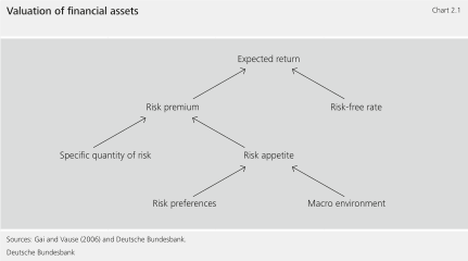
**Investors' risk appetite is a key concept in the valuation of financial assets.** To illustrate this, it is helpful to break down the expected return on financial assets into a risk-free and a risky component, the risk premium.[\[3\]](#_ftn_root_3) The risk premium consists of the quantity of risk associated with a specific asset and the market price per unit of risk (see Chart 2.1). A security's quantity of risk depends on the type of financial instrument and its specific characteristics. For example, investors demand risk compensation for various types of risk in fixed income securities, such as interest rate risk, liquidity risk and default risk. The amount of this compensation depends on specific characteristics of the bond, such as its maturity and the creditworthiness of the issuer. In addition, the size of the risk premium demanded by investors for all securities in an economy depends on the market price of risk. Risk appetite, the willingness of investors to take risks, is commonly defined as the inverse of the market price of risk (see the supplementary information entitled "[Derivation of the risk premium and risk appetite](#Derivation-of-the-risk-premium-and-risk-appetite)").[\[4\]](#_ftn_root_4) If investors are more willing to take risks, it means that they accept a lower risk premium on all financial assets in an economy, meaning that the market price of risk falls. This makes risk appetite a key concept in the valuation of financial assets. Risk appetite itself depends on two factors. The first is investors' risk preferences, which reflect the extent to which they disregard uncertainty about the future level of their consumption expenditure. Second, the general macroeconomic environment plays a crucial role as it influences the level of this uncertainty.[\[5\]](#_ftn_root_5){#par-ia8u96}
{#par-ueioa4}
Derivation of the risk premium and risk appetite
------------------------------------------------
**The risk premium is the product of an asset-specific quantity of risk and the market price of risk.** According to traditional asset pricing theory, in efficient, complete and arbitrage-free markets with rational investors and perfect information, the price \\( p_{i,t} \\) of a given asset \\( i \\) in \\( t \\) equals the present value of the future payoff of that asset \\( x_{i,t+1} \\) in \\( t+1 \\).[\[1\]](#_ftn_4fd69667_1) The future payoff \\( x_{i,t+1} \\) derives from the future price of the asset \\( p_{i,t+1} \\) and a potential dividend \\( d_{i,t+1} \\), meaning \\( x_{i,t+1} = p_{i,t+1} + d_{i,t+1} \\). This relationship is shown in the basic price equation (1).{#par-io9976}
$$ p_{i,t} = E_t(m_{t+1}\\cdot x_{i,t+1}). \\tag{$1$} $${#par-o8eai9}
The present value is determined using a discount factor, \\(m_{t+1}\\), which is stochastic and mainly depends on the risk preferences of investors and the macroeconomic environment. Under the given assumptions, the stochastic discount factor is unique and the same for all financial assets in an economy. {#par-o34749}
It is common practice to express price equation (1) in gross returns, \\( R_{i,t+1} = \\frac{x_{i,t+1}}{p_{i,t}} \\), by dividing by \\( p_{i,t} \\): {#par-u72a2i}
$$ 1 = E_t(m_{t+1}\\cdot R_{i,t+1}). \\tag{$2$} $$
Equation (2) implies that the expected value of the stochastic discount factor \\( E_t(m_{t+1}) \\) equals the risk-free discount factor \\( \\frac{1}{R_{f,t}} \\), where \\( R_{f,t} \\) is the risk-free interest rate known in \\( t \\).{#par-auo5i9}
Applying the shift rule for covariance results in:{#par-ei29ue}
$$ 1 = E_t(m_{t+1}) E_t(R_{i,t+1})+cov_t(m_{t+1}, R_{i,t+1}), \\tag{$3$} $${#par-a8o869}
and using \\( R_{f,t} = \\frac{1}{ E_t(m_{t+1})} \\) gives:{#par-o641u6}
$$ E_t(R_{i,t+1}) -- R_{f,t} = -cov_t(m_{t+1}, R_{i,t+1})\\cdot R_{f,t}. \\tag{$4$} $${#par-a8e1ao}
Equation (4) states that the expected risk premium of a risky asset, the difference between the expected gross return and the risk-free interest rate, is proportional to the covariance, multiplied by minus one, between the state-dependent return on the asset and the stochastic discount factor. Intuitively, the covariance describes the systematic fluctuations of the return \\( R_{i,t+1} \\) of the asset with investors' risk preferences and the macroeconomic environment. {#par-i327oe}
The risk premium, \\( E_t(R_{i,t+1}) -- R_{f,t} \\), can now be expressed as the product of the asset-specific quantity of risk, \\( \\beta_i \\), and the market price of risk, \\( \\lambda_t \\),{#par-o9oe75}
$$ E_t(R_{i,t+1}) -- R_{f,t} = \\left( \\underbrace{ \\frac{-cov_t(m_{t+1}, R_{i,t+1})}{var_t(m_{t+1})}}_{\\equiv \\beta_i} \\right) \\cdot \\left( \\underbrace{var_t(m_{t+1})\\cdot R_{f,t}}_{=\\lambda_t} \\right) = \\beta_i \\lambda_t. \\tag{$5$} $${#par-oioe8o}
**Risk appetite is defined as the inverse of the market price of risk.** Under the above assumptions, the market price of risk, \\( \\lambda_t \\), is the same for all assets in an economy and describes the risk premium demanded by investors for each unit of risk that they hold in equilibrium. In the literature, it is common to refer to the inverse of the market price of risk as risk appetite -- that is, investors' willingness to take on risk.[\[2\]](#_ftn_4fd69667_2) When risk appetite increases, meaning investors grow more willing to take on risk, the risk premium demanded by investors for each unit of risk falls. Thus, the market price of risk, and consequently risk appetite, depend on the macroeconomic environment and the risk preferences of investors.{#par-u613ao}
1. {#_ftn_4fd69667_1} See Cochrane (2005) and Deutsche Bundesbank (2016).
2. {#_ftn_4fd69667_2} See Gai and Vause (2006).
**Risk appetite in the euro area can be measured using empirical methods.** To this end, this analysis uses a new daily and broad-based risk appetite index for the euro area (see the supplementary information entitled "[Deriving an index to measure the risk appetite of euro area investors](#Deriving-an-index-to-measure-the-risk-appetite-of-euro-area-investors)").[\[6\]](#_ftn_root_6) This index measures investors' risk appetite by using principal component analysis to extract the common daily variation of individual risk measures from five asset segments.[\[7\]](#_ftn_root_7) The new index explains a large proportion of the common variation of the relevant risk measures for European stocks and bonds. It therefore appears well suited to contextualising developments in the euro area and comparing them with global or measures. This assessment is further supported by the index's close correlation with another indicator that measures risk appetite based on valuation differences between volatile and low-volatility stocks at the quarterly data level (see the supplementary information entitled "[Using valuation differences between volatile and low-volatility stocks to measure risk appetite](#Using-valuation-differences-between-volatile-and-low-volatility-stocks-to-measure-risk-appetite)").{#par-ao2273}
**Risk appetite in the euro area is time-varying and moves in line with the business cycle** (see Chart 2.2)**.** Specifically, the indicator shows that investors' risk appetite decreases in tandem with adverse macroeconomic developments, such as during the global financial crisis or the -19 pandemic. The decline in risk appetite leads investors to demand higher risk premia for holding the same quantity of risk associated with risky assets. Research suggests that, particularly in such crisis environments, the risk aversion of households and financial intermediaries can increase considerably.[\[8\]](#_ftn_root_8) Accordingly, households increasingly shy away from exposure to risky assets in order to secure their desired level of consumption during crises.[\[9\]](#_ftn_root_9) Such environments also typically lead to valuation losses. Valuation losses reduce the assets of economic agents, thus narrowing their scope for borrowing and lending. They face what are known as balance sheet constraints. This can, in particular, limit the risk-bearing capacity of financial intermediaries and thus increase their risk aversion.[\[10\]](#_ftn_root_10) Moreover, economic uncertainty typically increases in an adverse macro environment, contributing to a decline in risk appetite.[\[11\]](#_ftn_root_11) {#par-e242o3}
{#par-oe2183}
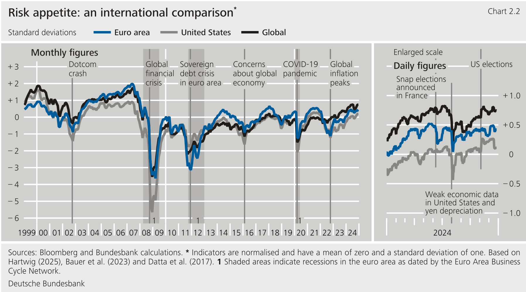
**The risk appetite index for the euro area tends to move in line with global financial market developments.** The high degree of co-movement between the risk appetite index in the euro area and the corresponding indices for or global risk appetite suggests that, to a large extent, globally active investors determine risk appetite in the euro area (see Chart 2.2).[\[12\]](#_ftn_root_12) At the same time, the indicator highlights episodes in which risk appetite in the euro area deviates from global developments. For example, this was the case during the European sovereign debt crisis from 2010 to 2012. At that time, investors were concerned about the sustainability of government debt in some euro area member countries and the economic outlook for the euro area. Risk appetite in the euro area fell significantly as a result, contributing to European stocks and corporate bonds coming under much greater pressure than those in the United States or at the global level. In addition, the daily availability of the euro area indicator proves useful for contextualising current financial market developments in real time (see Chart 2.2). One example of this is the risk-off movement in the euro area, an investment shift from riskier assets to safer assets, following the announcement of snap parliamentary elections in France in June 2024. The associated decline in risk appetite remained largely confined to the euro area. It therefore put pressure almost exclusively on European financial markets, with global financial markets and risk appetite measures proving robust.{#par-aai4ai}
Deriving an index to measure the risk appetite of euro area investors
---------------------------------------------------------------------
**The indicator presented here measures euro area investors' risk appetite based on the common daily change in 13 individual indicators from five different asset classes (see Table 2.1).** [\[1\]](#_ftn_4ca898ea_1) Risk appetite, defined as the inverse of the market price of risk, is theoretically the same for all financial assets in an economy of arbitrage-free and complete financial markets. So when risk appetite changes, the risk premia on all risky assets and thus their prices change. Given that risk appetite is reflected equally in all risk premia, it can be derived from individual indicators using principal component analysis.[\[2\]](#_ftn_4ca898ea_2) In this exercise, 13 individual indicators are used. They are key benchmarks for euro area financial markets and reflect not only asset-specific risk but also general risk appetite. Daily risk appetite is defined here as the first principal component of the standardised daily change in these 13 individual indicators. By definition, the first principal component explains the highest share of the total variance.[\[3\]](#_ftn_4ca898ea_3) All in all, at over 30%, the first principal component explains a considerable share of the common variation of these individual indicators and thus significantly more than other risk (appetite) indicators.[\[4\]](#_ftn_4ca898ea_4) The index is normalised so that a rise in the index corresponds to an increase in risk appetite. The level of risk appetite is calculated as the standardised sum of daily index values.[\[5\]](#_ftn_4ca898ea_5){#par-oe8953}
**The risk appetite indicator for the euro area is a broad measure that reflects risk measures in equity and bond markets to a similarly strong degree.**All 13 individual indicators contribute to the risk appetite indicator with the expected sign (Table 2.1). Accordingly, an increasing risk appetite is associated with rising stock prices, declining financial market volatility, narrower yield spreads and a depreciation in currencies that act as safe havens against the euro (US dollar and Swiss franc). The equity market-related variables (the two equity indices and the VSTOXX volatility index) have the highest weight in the index, followed by the yield spreads on corporate bonds (Table 2.1, column 2). Overall, according to a variance analysis, the equity and bond market variables explain a similarly large share of the daily common variation of these indicators (Table 2.1, column 3).{#par-a51ee3}
{#par-o38736}{#par-eu7923}{#par-u4eo43}{#par-i87u8a}{#par-aiu11a}{#par-ae661e}{#par-i74136}{#par-oui7oa}{#par-i5887e}{#par-ao9885}{#par-e69285}{#par-ou8ie8}{#par-e1a464}{#par-i6u926}{#par-ai5385}{#par-e4ou96}{#par-aoo433}{#par-ie25ou}
|----------------------------------------------------------------------------|-----------------------|--------------------------|
| **Table 2.1 Components of the daily risk appetite index for the euro area** |||
| **Financial market indicators** | **Index coefficient** | **Covariance share (%)** |
| **Equity market** | **.** | **34.43** |
| EURO STOXX index | 0.41 | 17.12 |
| EURO STOXX Banks index | 0.42 | 17.31 |
| **Volatility** | **.** | **19.65** |
| Implied volatility of the EURO STOXX 50 in 30 days (VSTOXX)^1^ | − 0.37 | 14.03 |
| Implied volatility of Bund future options with a maturity of three months | − 0.11 | 1.29 |
| Implied volatility of euro- dollar options with a maturity of three months | − 0.21 | 4.33 |
| **Government bonds** | **.** | **11.02** |
| Spread of ten-year -weighted bonds^2^ | − 0.29 | 8.34 |
| Spread dispersion of ten-year bonds^2^ | − 0.16 | 2.68 |
| **Corporate bonds** | **.** | **30.08** |
| iBoxx euro area spread (7‑10 years)^3^ | − 0.30 | 8.98 |
| iBoxx euro area BBB spread (7‑10 years)^3^ | − 0.34 | 11.28 |
| BofA euro area high-yield option-adjusted spread (all maturities) | − 0.31 | 9.83 |
| **Foreign exchange market** | **.** | **4.81** |
| Exchange rate of the dollar against the euro^4^ | − 0.11 | 1.21 |
| Exchange rate of the Swiss franc against the euro^4^ | − 0.17 | 2.92 |
| Euro- dollar basis for 3-month money market operations^5^ | − 0.09 | 0.78 |
| Sources: Bloomberg and Bundesbank calculations. The index coefficient (column 2) indicates the weight that each individual indicator takes within the risk appetite index for the euro area (the components of the first eigenvector of the correlation matrix of the 13 financial market indicators). Stock prices and exchange rates are included in the index as daily logarithmic price differences; volatility indicators are daily changes measured in index points; bond spreads and their dispersion are daily changes measured in percentage points. The sign of the risk appetite index is normalised such that an increase in the index corresponds to an increase in risk appetite. The covariance share (column 3) is defined as the covariance of the respective standardised individual indicator with the daily change in the risk appetite index divided by the variance of the daily change in the risk appetite index. The covariance shares add up to one. **1** The VSTOXX has been available since 1 January 2007; earlier values are taken from the VDAX. **2** Spreads relative to the yield on ten-year Bunds. **3** Spreads relative to the matched-maturity Bund yield as measured by the corresponding iBoxx index. The iBoxx data have been available since 23 May 2002; earlier values are taken from the corresponding BofA indices and the ten-year Bund yield. **4** An increase in the exchange rate corresponds to a depreciation in the euro against its partner currency. **5** An increase in the swap basis corresponds to higher dollar financing costs for banks in the euro area through foreign exchange swaps compared with direct refinancing in the money markets; see also Deutsche Bundesbank (2022). |||
{#par-u4i5ao}
1. {#_ftn_4ca898ea_1} See Hartwig (2025).
2. {#_ftn_4ca898ea_2} See Miranda-Agrippino and Rey (2020) as well as Bauer et al. (2023). Principal component analysis is an established statistical method for capturing the information within a dataset with a small number of ideally meaningful linear combinations of the principal components.
3. {#_ftn_4ca898ea_3} The first principal component is determined using the first eigenvector of the correlation matrix of the 13 financial market indicators and the standardised data, which have a mean of zero and a standard deviation of one.
4. {#_ftn_4ca898ea_4} The corresponding indicators for and global risk appetite explain 13% and 20%, respectively, of the common variation of individual indicators for the euro area. The Bloomberg and Goldman Sachs financial conditions indices explain only around 7% and 13% of the common variation, respectively.
5. {#_ftn_4ca898ea_5} The indicator thus has a mean of zero and a standard deviation of one.
Using valuation differences between volatile and low-volatility stocks to measure risk appetite
-----------------------------------------------------------------------------------------------
**This supplementary information presents, in the sense of a robustness analysis, an alternative measure of risk appetite (the price of volatile stocks, or** ),**defined as the book-to-market ratio of low-volatility stocks minus the book-to-market ratio of high-volatility stocks.** Expanding on the existing body of literature for the United States, the measure is also calculated for the euro area.[\[1\]](#_ftn_492f8623_1) Overall, the analysis indicates that the measure in both currency areas correlates relatively closely with the corresponding risk appetite indices based on principal component analyses (see the [supplementary information on deriving an index to measure the risk appetite of investors in the euro area for details on the risk appetite index for the euro area](#Deriving-an-index-to-measure-the-risk-appetite-of-euro-area-investors)) and with key macro variables as well. As a result, this supports the robustness of the analysis using the principal component risk appetite indices described above. {#par-i3ea7e}
**The study builds on a broad corporate dataset for the euro area and the United States.** The sample comprises all enterprises that have been included in the Euro Stoxx or S\&P 500 at least once at the beginning of the year in the observation period since 1999.[\[2\]](#_ftn_492f8623_2) In total, there are 640 European and 1,064 enterprises. The measure is calculated in quarterly data.{#par-e73698}
**The** **measure is defined as the difference between the (arithmetic) average book-to-market (BM) ratio of low-volatility stocks and the (arithmetic) average BM ratio of high-volatility stocks.** This measure is calculated by sorting all the stocks into five volatility quintiles at the end of each quarter.[\[3\]](#_ftn_492f8623_3) Stocks in the lowest (highest) volatility quintile are defined as low volatility (high volatility). The measure is based on the intuition that highly volatile stocks should be particularly sensitive to changes in risk appetite. Furthermore, in terms of their investment behaviour, these enterprises can be expected to resemble many unlisted enterprises that significantly shape the aggregate economy.[\[4\]](#_ftn_492f8623_4) Their valuation should therefore visibly reflect the risk appetite relevant to the economy as a whole. For example, when the prices of high-volatility stocks increase, their BM ratio declines. Assuming the BM ratio of low-volatility stocks remains comparatively stable, this will raise the measure, thus indicating that investors are more willing to take risks.{#par-o659au}
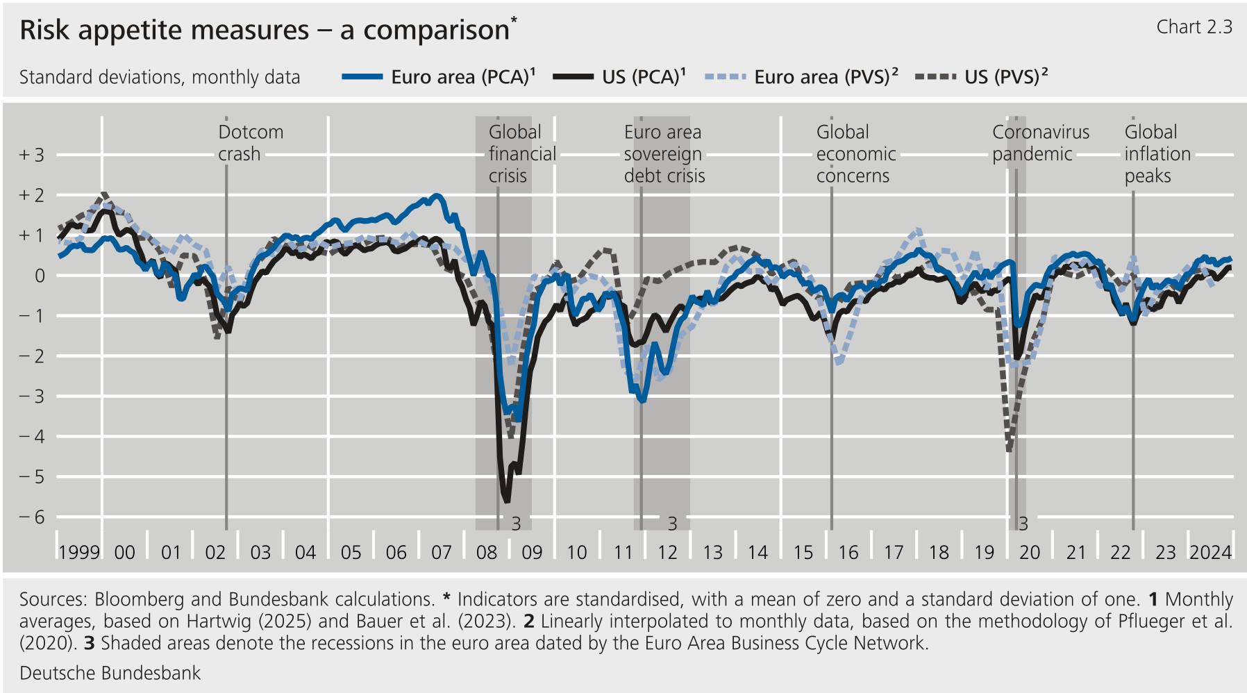
**The** **measure is closely correlated with the principal component risk appetite indices.** Comparing the measure with other relevant risk measures helps to put it into context. The comparison observes not just the principal component risk appetite indices described above, but also measures of volatility in equity and sovereign bond markets.[\[5\]](#_ftn_492f8623_5) The comparison furthermore takes into account a measure that reflects the dispersion of earnings estimates of enterprises with high-volatility and low-volatility stock prices.[\[6\]](#_ftn_492f8623_6) According to the comparison based on a correlation analysis, the measure on both sides of the Atlantic is the measure that correlates the closest with the corresponding risk appetite indices derived from principal component analysis (euro area: ρ=0.65, United States: ρ=0.80). The correlation between the indicators and the dispersion of earnings estimates and volatility indicators is somewhat weaker and, as expected, negative. {#par-i92ao2}
**The** **measure likewise correlates with key macro variables like the real rate of interest and reflects new macroeconomic information.** The coefficient of a simple linear regression of the measure for the respective currency area on the corresponding one-year real rate of interest is positive and significant in each case. This would suggest that a stronger risk appetite is usually associated with stronger growth, meaning that risk appetite can also be interpreted as a cyclical indicator. This proposition is also supported by the positive correlation that likewise exists between the measure and upside surprises in growth or corporate earnings growth.[\[7\]](#_ftn_492f8623_7){#par-a35a68}
**In some cases, the** **measures signal transatlantic differentials in risk appetite.** The measure for the euro area fell notably as a result of the financial and sovereign debt crisis, the membership referendum in the United Kingdom in 2016, and the outbreak of the pandemic in 2020 (see Chart 2.3). Following the onset of the war in Ukraine in 2022, it declined at a relatively measured pace. The measure for the United States fell more strongly still during the financial crisis and the pandemic, but proved to be relatively robust to the European sovereign debt crisis and Brexit. Much like the measure based on principal component analysis, then, the measure helps to identify the euro area-specific risk appetite and to put it into an international context.{#par-a66o67}
{#par-a66o67}
1. {#_ftn_492f8623_1} The measure of risk appetite was first presented by Pflueger et al. (2020) for enterprises.
2. {#_ftn_492f8623_2} In the euro area, only enterprises in the Euro Stoxx since 2002 are included. Furthermore, one-quarter-ahead stock prices and the book-to-market ratio must be available for these firms.
3. {#_ftn_492f8623_3} Volatility is based on stock returns in the past two months (44 days) and is fed into the measure provided there are at least 20 stock return observations in the past two months.
4. {#_ftn_492f8623_4} See Pflueger et al. (2020).
5. {#_ftn_492f8623_5} For equity markets, the options-implied volatility of the Euro Stoxx and S\&P 500 are used as measures of stock volatility. For sovereign bond markets, the implied volatility of German and sovereign bonds is observed (the volatility of Bund futures and the index).
6. {#_ftn_492f8623_6} This dispersion measure is constructed in much the same way as the measure. It is calculated by first determining enterprise-level risk in the form of the normalised dispersion of 12-month earnings estimates, as sourced from I/B/E/S analyst estimates. The aggregated dispersion measure is the median of this risk for enterprises with highly volatile stock prices (highest volatility quintile) less the median of this risk for enterprises with low-volatility stock prices (lowest volatility quintile).
7. {#_ftn_492f8623_7} Surprises are defined here as deviations in realised values from the corresponding survey-based expectations (: estimates by Consensus Economics; corporate earnings: I/B/E/S analyst estimates).
2 Monetary policy and financial markets
---------------------------------------
**Monetary policy influences the prices of financial assets via various transmission channels.** When the central bank raises policy rates in response to an overheating economy, risk-free interest rates with longer maturities will generally rise as well.[\[13\]](#_ftn_root_13) This reduces the present value of future cash flows and, thus, the prices of financial assets. In addition, tighter monetary policy reduces firms' expected profits through its dampening impact on economic activity, which further depresses asset prices. Ultimately, investors can demand higher risk premia if policy rates rise unexpectedly, because specific quantities of risk increase by different amounts. In particular, investors demand higher risk premia from those enterprises whose default risk goes up in a weaker economic environment. And lastly, monetary policy tightening can reduce risk appetite in financial markets.[\[14\]](#_ftn_root_14){#par-a483oe}
**Monetary policy tightening can increase investors' risk appetite through heightened uncertainty and decreased risk aversion.** [\[15\]](#_ftn_root_15) Risk aversion may go up as a result of a monetary policy-induced rise in risk-free interest rates. This is based on the idea that investors with predefined nominal return targets can achieve the same expected total return on their portfolio if they shift into risk-free assets. As a result, this group of investors reduces the share of risky assets in their portfolios. Other investors now have to hold the riskier assets that were sold and are only willing to do so in return for a higher risk premium.[\[16\]](#_ftn_root_16) Moreover, tighter monetary policy dampens consumption levels and economic prospects. This makes investors more risk-averse. A monetary policy-induced increase in risk-free interest rates can also cause economic agents to run into the greater balance sheet constraints explained above. Together with the aforementioned effects on economic activity, this can elevate economic uncertainty.[\[17\]](#_ftn_root_17){#par-iu5ua3}
**Using an event study, the following sections of this article explore how monetary policy measures affect euro area financial markets via the risk-taking channel.** To this end, monetary policy surprise components directly connected with the Governing Council of the 's monetary policy decisions are identified.[\[18\]](#_ftn_root_18) These monetary policy surprise components are then used in an event study to empirically analyse the response of the risk appetite index together with the prices of risky assets, risk-free interest rate expectations and selected exchange rates against the euro over time. According to the event study, market participants' short to medium-term interest rate expectations, measured by the response of the two-year euro area rate, increase by 25 basis points following an unexpected restrictive monetary policy impulse from the Eurosystem (see Chart 2.4).{#par-o9ea37}
{#par-a52ie8}
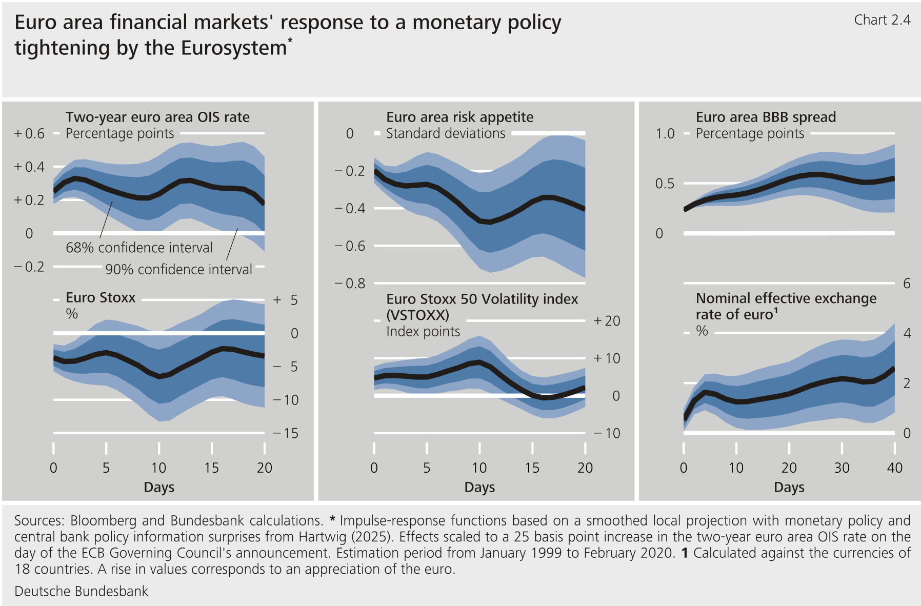
**An unexpected monetary policy tightening by the Eurosystem triggers a persistent and economically significant risk-off movement in financial markets.**This is reflected in declining equity prices, higher equity market volatility and larger spreads on corporate bonds. In addition, investors' risk appetite decreases and continues to dwindle over time. This implies that the impact of monetary policy on investors' risk appetite is not just limited to the short term. Rather, the results suggest that it amplifies the risk-off movement of equities and bonds over time, thus indicating that the risk-taking channel has an economically significant effect in the transmission of monetary policy. This topic is examined below.{#par-o3iaao}
**The risk-taking channel plays an important role in the transatlantic transmission of monetary policy** (see the supplementary information entitled "[Transatlantic transmission of monetary policy and the role of risk appetite](#Transatlantic-transmission-of-monetary-policy-and-the-role-of-risk-appetite)"). The monetary policy measures of the Federal Reserve cause persistent movements in euro area financial markets. Empirical analysis suggests that these developments are largely transmitted through the risk-taking channel of globally active investors. The Eurosystem's monetary policy also influences investors' risk appetite. However, its impact on financial markets is markedly weaker overall than the impact of monetary policy on euro area financial markets. Moreover, investors' risk appetite also influences movements in the exchange rate of the euro against other currencies. Ceteris paribus, a rise in domestic risk-free interest rates induced by the Eurosystem's monetary policy leads to higher interest rate differentials vis-à-vis all other currency areas. This typically results in an appreciation of the nominal effective exchange rate of the euro.[\[19\]](#_ftn_root_19) However, the Eurosystem's monetary policy impulse also dampens the risk appetite of global investors. This could explain why the euro appreciates less strongly, or not at all, against the dollar, the Swiss franc and the yen. These currencies are either regarded as safe haven currencies or serve as financing currencies in speculative carry-trade transactions, which are increasingly unwound in times of heightened financial market tension.[\[20\]](#_ftn_root_20) The response of risk appetite thus tempers the appreciation pressure on the nominal effective euro.{#par-u9a489}
Transatlantic transmission of monetary policy and the role of risk appetite
---------------------------------------------------------------------------
**On days when monetary policy decisions are announced, the prices of risky assets often move in the same direction in the euro area and the United States, which suggests that the risk appetite of globally active investors is influenced by monetary policy.** Against this background, the supplementary information provided here uses an event study to examine how the monetary policy of the Eurosystem and the Federal Reserve () transmits transatlantically to financial markets, and what role investors' risk appetite plays in this context. To this end, monetary policy surprise components are identified in direct connection with the respective central bank's monetary policy decisions. These monetary policy surprises are then used in an event study to empirically examine the response of key financial market indicators over time.{#par-eiiouu}
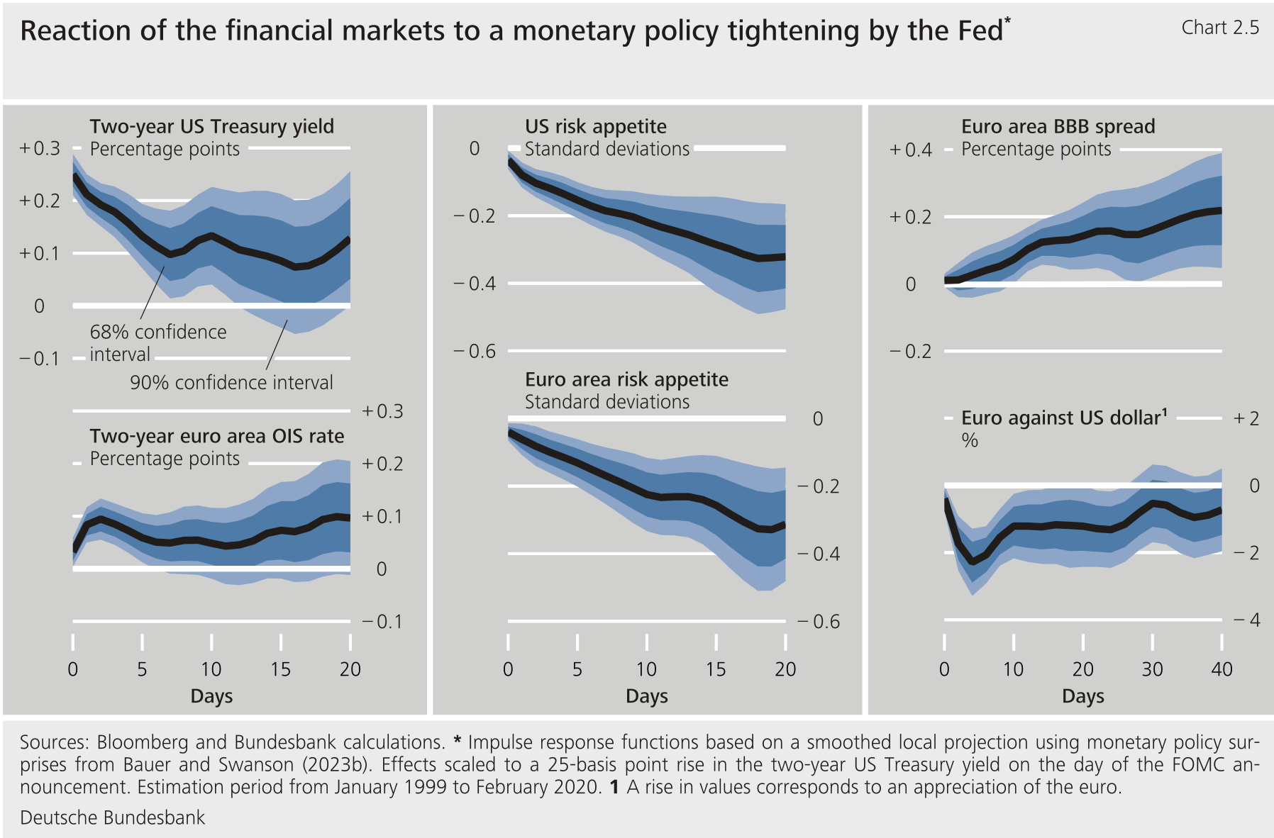
**The risk appetite channel significantly contributes to the influence of** **monetary policy on European financial markets** (Chart 2.5)**.** An approach that is well established in the literature is used to identify the Fed's monetary policy surprises.[\[1\]](#_ftn_4600b0ec_1) The results of the event study show that monetary policy has a substantial impact on financial markets on both sides of the Atlantic via the risk appetite channel: an unexpected tightening of 25 basis points by the is accompanied in both currency areas by a persistent and economically significant risk-off movement in equity and bond markets. This is reflected in the fact that the impulse from the dampens risk appetite in both currency areas, albeit with stronger effects in the domestic market. Furthermore, tighter monetary policy causes a noticeable deprecation of the euro against the dollar. In addition to the widened interest rate differential between the United States and the euro area, the decline in investors' risk appetite may contribute to the marked depreciation of the euro against the dollar via safe haven effects. Accordingly, the reduced risk appetite of global investors bolsters demand for assets in safe haven currency areas like the United States, which intensifies the depreciation of the euro against the dollar.[\[2\]](#_ftn_4600b0ec_2) Moreover, the study results show a marked appreciation of the euro against the Canadian and the Australian dollar. This effect can also be linked to the decline in risk appetite, as these currencies are often targets for speculators.[\[3\]](#_ftn_4600b0ec_3) As a result of these partially opposing movements against individual currencies, the depreciation of the nominal effective euro is weaker than without this effect.{#par-eoa638}
{#par-i788o8}
**A monetary policy tightening by the Eurosystem reduces** **investors' risk appetite and triggers a moderate risk-off movement in** **financial markets.** For this event study, the monetary policy surprise components of the Governing Council presented in the main text are considered.[\[4\]](#_ftn_4600b0ec_4) Compared with the effects of a monetary policy impulse in the United States on the euro area, the study finds that an unexpected monetary policy tightening by the Governing Council only strongly delays, but hardly significantly increases, short to medium-term interest rate expectations. Nonetheless, it does trigger a moderate risk-off movement in equity and bond markets and also leads to a lasting reduction in investors' risk appetite. This demonstrates that the Eurosystem's monetary policy influences asset prices via the risk appetite channel, too. In addition, the euro appreciates less sharply against the dollar than against a broad basket of currencies despite a widening of the euro- dollar interest rate differential. This response is consistent with the risk appetite channel. In particular, a decline in risk appetite bolsters demand for Treasuries, which gives the dollar an additional boost. In effect, the risk appetite channel thus weakens the impulse from the Eurosystem's monetary policy tightening on Treasury yields and the appreciation of the euro against the dollar.{#par-uo1262}
1. {#_ftn_4600b0ec_1} See Hartwig (2025).
2. {#_ftn_4600b0ec_2} See Miranda-Agrippino and Rey (2020) as well as Bauer et al. (2023). Principal component analysis is an established statistical method for capturing the information within a dataset with a small number of ideally meaningful linear combinations of the principal components.
3. {#_ftn_4600b0ec_3} The first principal component is determined using the first eigenvector of the correlation matrix of the 13 financial market indicators and the standardised data, which have a mean of zero and a standard deviation of one.
4. {#_ftn_4600b0ec_4} The corresponding indicators for and global risk appetite explain 13% and 20%, respectively, of the common variation of individual indicators for the euro area. The Bloomberg and Goldman Sachs financial conditions indices explain only around 7% and 13% of the common variation, respectively.
3 Macroeconomic effects of monetary policy and risk appetite
------------------------------------------------------------
**Unlike in the United States, the Eurosystem's risk-taking channel can amplify a monetary policy tightening impulse through higher risk premia and dampen it through exchange rate movements.** When risk appetite falls as a result of monetary policy tightening, risk premia and thus the financing costs of economic agents can rise above the risk-free level. Rising risk premia can also amplify losses in asset values. At the same time, the decline in risk appetite can weaken the effectiveness of the Eurosystem's monetary policy tightening via the exchange rate channel. In particular, diminishing risk appetite can dampen demand for euro-denominated assets and counteract an appreciation of the euro. The question of which aspect dominates is ultimately an empirical one. Below, the role of the risk-taking channel for monetary policy transmission is examined using an estimated dynamic macro-financial model in order to quantify the effects for the euro area.[\[21\]](#_ftn_root_21){#par-ie899i}
**The estimation results show that tighter monetary policy reduces economic activity, the price level and investors' risk appetite** (see Chart 2.6)**.** The impact of monetary policy on risk premia plays a key role. Rising policy rates are accompanied by higher risk premia, as measured by the spreads on euro area BBB-rated corporate bonds. These increase the cost of capital beyond the rise in risk-free interest rates. At the same time, tighter monetary policy leads to an effective appreciation of the euro against the currencies of 18 trading partners. This reflects the fact that a wider interest rate differential causes foreign investors to increasingly seek out risk-free euro-denominated assets. {#par-e684e7}
{#par-o667a6}
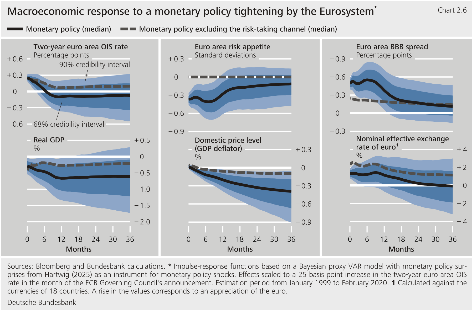
**The risk-taking channel increases the effectiveness of the Eurosystem's monetary policy measures on economic activity and prices, as shown by a counterfactual analysis.** Using a counterfactual analysis, it is possible to isolate the impact of monetary policy measures. The analysis looks at how the variables behave under the assumption that monetary policy does not affect investors' risk appetite.[\[22\]](#_ftn_root_22) The results show that real economic activity and domestic price levels would each be significantly less dampened than in a scenario in which monetary policy does affect investors' risk appetite (grey dashed lines vs. black solid lines). In the absence of an effective risk-taking channel, monetary policy tightening causes the nominal effective exchange rate of the euro to appreciate more strongly owing to the effects outlined above. Taken in isolation, this would increase the dampening effect of tighter monetary policy on economic activity and prices. However, in this counterfactual scenario, risk premia would also rise less sharply and equity prices would not fall by as much, which would dampen the effectiveness of monetary policy via the cost of capital channel and asset price effects. Overall, the latter two channels outweigh the opposing effect of the exchange rate movement. The risk-taking channel thus strengthens the effectiveness of the Eurosystem's monetary policy measures on economic activity and prices.{#par-oa79i4}
4 Conclusions and outlook
-------------------------
**Analysing investors' risk appetite provides valuable information for assessing financial market developments and the effects of monetary policy.**This article looks at a new broad-based risk appetite index based on daily data for the euro area. The risk appetite index is time-varying, moves in line with the business cycle, and is co-determined by monetary policy. While it has generally moved in tandem with global financial market developments, it has shown significant responses to euro area-specific stress situations and monetary policy changes. {#par-i75o42}
**The risk-taking channel, the tendency of monetary policy to influence investors' risk appetite, has a significant impact on the effectiveness of the Eurosystem's monetary policy on the macroeconomy and financial markets.**The risk-taking channel interacts with other monetary policy transmission channels. For example, it reinforces the restrictive effect of a tightening of Eurosystem monetary policy via the cost of capital and asset price channels by reducing investors' risk appetite, but diminishes the restrictive impulse via the exchange rate channel. An empirical study of these effects shows that the former effects predominate, which means that the risk-taking channel overall strengthens the dampening impact of monetary policy tightening on economic activity and the general price level. {#par-e7uoa2}
**The risk-taking channel contributes to the transmission of monetary policy impulses between currency areas, not only from the United States to the euro area, but also -- to a lesser extent -- from the euro area to the United States.** The event study outlined here complements existing literature on the relevance of the risk-taking channel for monetary policy. It shows that a tightening of monetary policy by the Eurosystem also results in a swift and persistent risk-off movement in international financial markets and reduces risk appetite on both sides of the Atlantic. {#par-u6e253}
**The analyses presented in this article suggest that, between July 2022 and September 2023, the dynamic economic environment weakened the dampening effect of monetary policy on risk appetite.** The results indicate that, taken in isolation, the monetary policy tightening cycle is likely to have dampened risk appetite among investors. However, in a dynamic economic environment, risk appetite has proved robust overall since autumn 2022, meaning that the restrictive monetary policy impulses were not intensified by rising risk premia in individual financial market segments. {#par-u1e9oe}
**Looking ahead, the results could be extended along further dimensions.** For instance, the way in which the risk appetite index was designed does not allow us to quantify the extent to which monetary policy influences risk appetite via a change in risk aversion or a change in economic uncertainty. However, a distinction such as this is important for modelling the intertemporal consumption and investment decisions of economic agents.{#par-ai688e}
List of references
------------------
Acharya, V. and H. Naqvi (2012), [The seeds of a crisis: A theory of bank liquidity and risk taking over the business cycle](https://www.sciencedirect.com/science/article/pii/S0304405X12000967), Journal of Financial Economics, 106(2), pp. 349‑366.{#par-i36587}
Adrian, T. and H. S. Shin (2010), [Liquidity and leverage, Journal of Financial Intermediation](https://www.sciencedirect.com/science/article/pii/S1042957308000764), 19(3), pp. 418‑437.{#par-a1o28a}
Adrian, T., F. Duarte and T. Iyer (2023), [The market price of risk and macro-financial dynamics](https://www.imf.org/-/media/Files/Publications/WP/2023/English/wpiea2023199-print-pdf.ashx), International Monetary Fund, Working Paper, 23199.{#par-eoi8a8}
Antolín-Díaz, J., I. Petrella and J. F. Rubio-Ramírez (2021), [Structural scenario analysis with](https://www.sciencedirect.com/science/article/pii/S0304393220300751), Journal of Monetary Economics, 117, pp. 798‑815.{#par-o3u956}
Baele, L., G. Bekaert, K. Inghelbrecht and M. Wei (2020), [Flights to safety](https://academic.oup.com/rfs/article/33/2/689/5512368), The Review of Financial Studies, 33(2), pp. 689‑746.{#par-a3o744}
Baker, S. R., N. Bloom and S. J. Davis (2016), [Measuring economic policy uncertainty](https://academic.oup.com/qje/article/131/4/1593/2468873?login=true), The Quarterly Journal of Economics, 131(4), pp. 1593‑1636.{#par-u36eai}
Bansal, R. and A. Yaron (2004), [Risks for the long run: A potential resolution of asset pricing puzzles](https://onlinelibrary.wiley.com/doi/full/10.1111/j.1540-6261.2004.00670.x), Journal of Finance, 59(4), pp. 1481‑1509.{#par-i96e8i}
Bauer, M. D., B. S. Bernanke and E. Milstein (2023), [Risk appetite and the risk-taking channel of monetary policy](https://www.aeaweb.org/articles?id=10.1257/jep.37.1.77), Journal of Economic Perspectives, 37(1), pp. 77‑100.{#par-u2eu12}
Bauer, M. D. and E. T. Swanson (2023a), [An alternative explanation for the "Fed information effect"](https://www.aeaweb.org/articles?id=10.1257/aer.20201220), American Economic Review, 113(3), pp. 664‑700.{#par-a7u5i3}
Bauer, M. D. and E. T. Swanson (2023b), [A reassessment of monetary policy surprises and high-frequency identification](https://www.journals.uchicago.edu/doi/full/10.1086/723574), Macroeconomics Annual, 37(1), pp. 87‑155.{#par-e4i257}
Bekaert, G., M. Hoerova and M. Lo Duca (2013), [Risk, uncertainty and monetary policy](https://www.sciencedirect.com/science/article/pii/S0304393213000871), Journal of Monetary Economics, 60(7), pp. 771‑788.{#par-o9e6o8}
Bekaert, G., E. C. Engstrom and N. R. Xu (2022), [The time variation in risk appetite and uncertainty](https://pubsonline.informs.org/doi/abs/10.1287/mnsc.2021.4068), Management Science, 68(6), pp. 3975‑4004.{#par-oi2i34}
Bernanke, B. S. and K. N. Kuttner (2005), [What explains the stock market's reaction to Federal Reserve policy?](https://onlinelibrary.wiley.com/doi/full/10.1111/j.1540-6261.2005.00760.x), The Journal of Finance, 60(3), pp. 1221‑1257.{#par-e2687u}
Bloom, N. (2009), [The impact of uncertainty shocks](https://onlinelibrary.wiley.com/doi/abs/10.3982/ecta6248), Econometrica, 77(3), pp. 623‑685.{#par-au4i87}
Borio, C. and H. Zhu (2012), [Capital regulation, risk-taking and monetary policy: A missing link in the transmission mechanism?](https://www.sciencedirect.com/science/article/pii/S1572308911000611), Journal of Financial Stability, 8(4), [pp.](https://pubsonline.informs.org/doi/abs/10.1287/mnsc.2021.4068)[236‑251.](https://www.sciencedirect.com/science/article/pii/S1572308911000611){#par-eee29o}
Brave, B. and R. A. Butters (2012), [Diagnosing the financial system: Financial conditions and financial stress](https://www.ijcb.org/journal/ijcb12q2a6.htm), International Journal of Central Banking, 8, pp. 191‑239.{#par-aiu7e8}
Buch, C. M., S. Eickmeier and E. Prieto (2014), [In search for yield? Survey-based evidence on bank risk taking](https://www.sciencedirect.com/science/article/pii/S0165188914000281), Journal of Economic Dynamics and Control, 43, pp. 12‑30.{#par-au5132}
Campbell, J. Y. and J. H. Cochrane (1999), [By force of habit: A consumption‐based explanation of aggregate stock market behavior](https://www.journals.uchicago.edu/doi/abs/10.1086/250059), Journal of Political Economy, 107(2), pp. 205‑251.{#par-eo1978}
Campbell, J. Y. and R. Sigalov (2022), [Portfolio choice with sustainable spending: A model of reaching for yield](https://www.sciencedirect.com/science/article/pii/S0304405X21002002), Journal of Financial Economics, 143(1), pp. 188‑206.{#par-u55e3o}
Cieslak, A. and A. Schrimpf (2019), [Non-monetary news in central bank communication](https://www.sciencedirect.com/science/article/pii/S002219961830268X), Journal of International Economics, 118, pp. 293‑315.{#par-ai6391}
Cochrane, J. H. (2017), [Macro-finance](https://academic.oup.com/rof/article-abstract/21/3/945/3060346), Review of Finance, 21(3), pp. 945‑985.
Cochrane, J. H. (2005), Asset pricing, Princeton University Press.
Datta, D., J. M. Londono, B. Sun, D. Beltran, T. Ferreira, M. Iacoviello, M. R. Jahan-Parvar, C. Li, M. Rodriguez and J. Rogers (2017), [Taxonomy of global risk, uncertainty, and volatility measures](https://www.federalreserve.gov/econres/ifdp/taxonomy-of-global-risk-uncertainty-and-volatility-measures.htm), Board of Governors of the Federal Reserve System, International Finance Discussion Paper, 1216.{#par-eo71e3}
Deutsche Bundesbank (2023), [Term structures in economic analysis](https://www.bundesbank.de/content/903316), Monthly Report, January 2023.
Deutsche Bundesbank (2022), [The validity of interest parity in times of crisis](https://www.bundesbank.de/content/898764), Monthly Report, October 2022.{#par-i2uu6e}
Deutsche Bundesbank (2021), [The impact of monetary policy depending on the debt situation in the non-financial private sector: Evidence for the euro area](https://www.bundesbank.de/content/864102), Monthly Report, April 2021.
Deutsche Bundesbank (2018), [The importance of bank profitability and bank capital for monetary policy](https://www.bundesbank.de/content/667544), Monthly Report, January 2018.
Deutsche Bundesbank (2016), [Stock market valuations -- theoretical basics and enhancing the metrics](https://www.bundesbank.de/content/667076), Monthly Report, April 2016.
Deutsche Bundesbank (2014), [Exchange rates and financial stress](https://www.bundesbank.de/content/666616), Monthly Report, July 2014.
Gai, P. and N. Vause (2006), [Measuring investors' risk appetite](https://www.ijcb.org/journal/ijcb06q1a5.htm), International Journal of Central Banking, 2(1), pp. 167‑188.{#par-o2ua61}
Gertler, M. and P. Karadi (2015), [Monetary policy surprises, credit costs, and economic activity](https://www.aeaweb.org/articles?id=10.1257/mac.20130329), American Economic Journal: Macroeconomics, 7(1), pp. 44‑76.{#par-ui3963}
Haddad, V. and T. Muir (2021), [Do intermediaries matter for aggregate asset prices?](https://onlinelibrary.wiley.com/doi/full/10.1111/jofi.13086), The Journal of Finance, 76(6), pp. 2719-2761.{#par-u35io6}
Hanson, S. G., D. O. Lucca and J. H. Wright (2021), [Rate-amplifying demand and the excess sensitivity of long-term rates](https://academic.oup.com/qje/article/136/3/1719/6219101), The Quarterly Journal of Economics, 136(3), pp. 1719‑1781.{#par-u35io6}
Hartwig, B. (2025), Risk appetite and monetary policy in the euro area, mimeo. {#par-iuo81a}
He, Z. G. and A. Krishnamurthy (2013), [Intermediary asset pricing](https://www.aeaweb.org/articles?id=10.1257/aer.103.2.732), American Economic Review, 103(2), pp. 732‑770.{#par-a3i49a}
Hossfeld, O. and R. MacDonald (2015), [Carry funding and safe haven currencies: A threshold regression approach](https://www.sciencedirect.com/science/article/pii/S0261560615001205), Journal of International Money and Finance, 59, pp. 185‑202.{#par-a3ua93}
Jiménez, G., S. Ongena, J.-L. Peydró and J. Saurina (2014), [Hazardous times for monetary policy: What do twenty-three million bank loans say about the effects of monetary policy on credit risk-taking?](https://onlinelibrary.wiley.com/doi/abs/10.3982/ECTA10104), Econometrica, 82(2), pp. 463‑505.{#par-u394eo}
Jurado, K., S. C. Ludvigson and S. Ng (2015), [Measuring uncertainty](https://www.aeaweb.org/articles?id=10.1257/aer.20131193), American Economic Review, 105(3), pp. 1177‑1216.{#par-ai334u}
Kalemli-Özcan, Ṣ. (2019), [monetary policy and international risk spillovers](https://www.nber.org/papers/w26297), National Bureau of Economic Research, Working Paper, 26297.{#par-i4oeeo}
Kashyap, A. K. and J. C. Stein (2023), [Monetary policy when the central bank shapes financial-market sentiment](https://www.aeaweb.org/articles?id=10.1257/jep.37.1.53), Journal of Economic Perspectives, 37(1), pp. 53‑76.{#par-ea5354}
Kerssenfischer, M. (2022), [Information effects of euro area monetary policy](https://www.sciencedirect.com/science/article/pii/S0165176522001653), Economics Letters, 216, 110570.{#par-aa3u4o}
Ludvigson, S. C., S. Ma and S. Ng (2021), [Uncertainty and business cycles: Exogenous impulse or endogenous response?,](https://www.aeaweb.org/articles?id=10.1257/mac.20190171) American Economic Journal: Macroeconomics, 13(4), pp. 369‑410.{#par-ai6536}
Miranda-Agrippino, S. and H. Rey (2020), [U.S. Monetary policy and the global financial cycle](https://academic.oup.com/restud/article/87/6/2754/5834728), The Review of Economic Studies, 87(6), pp. 2754‑2776.{#par-i3o443}
Pflueger, C., E. Siriwardane and A. Sunderam (2020), [Financial market risk perceptions and the macroeconomy](https://academic.oup.com/qje/article/135/3/1443/5775315), The Quarterly Journal of Economics, 135(3), pp. 1443‑1491.{#par-ei9894}
Romer, C. D. and D. H. Romer (2000), [Federal Reserve information and the behavior of interest rates](https://www.aeaweb.org/articles?id=10.1257/aer.90.3.429), American Economic Review, 90(3), pp. 429‑457.{#par-i17a7e}
Stock, J. and M. Watson (2010), [Monthly estimates of real /: Research memorandum](https://www.princeton.edu/~mwatson/mgdp_gdi/Monthly_GDP_GDI_Sept19.pdf), Manuscript, Harvard University and Princeton University.{#par-e45467}
1. {#_ftn_root_1} See Borio and Zhu (2012), Adrian and Shin (2010), Acharya and Naqvi (2012), Bekaert et al. (2013), Jiménez et al. (2014), Buch et al. (2014).
2. {#_ftn_root_2} See Kalemli-Özcan (2019), Miranda-Agrippino and Rey (2020), Bauer et al. (2023).
3. {#_ftn_root_3} See Cochrane (2005), Deutsche Bundesbank (2016).
4. {#_ftn_root_4} See Gai und Vause (2006).
5. {#_ftn_root_5} Economic uncertainty can be measured as the standard deviation of consumption growth; see Cochrane (2005).
6. {#_ftn_root_6} See Hartwig (2025).
7. {#_ftn_root_7} See Miranda-Agrippino und Rey (2020), Bauer et al. (2023). For alternative approaches, see Brave und Butters (2012), Datta et al. (2017), Bekaert et al. (2022), Adrian et al. (2023).
8. {#_ftn_root_8} See Cochrane (2017) for an overview.
9. {#_ftn_root_9} See Campbell und Cochrane (1999).
10. {#_ftn_root_10} The risk-bearing capacity of financial intermediaries depends on, amongst other things, regulatory requirements and self-imposed risk limits. See Adrian und Shin (2010), He und Krishnamurthy (2013), Haddad und Muir (2021), Deutsche Bundesbank (2018, 2021).
11. {#_ftn_root_11} See Bansal und Yaron (2004). In addition to an adverse economic climate, economic uncertainty can also rise due to an increase in political uncertainty or asymmetric information on the value of risky assets; see Bloom (2009), Jurado et al. (2015), Baker et al. (2016), Ludvigson et al. (2021) and Adrian et al. (2023).
12. {#_ftn_root_12} See Miranda-Agrippino und Rey (2020). The correlation between the risk appetite measures is above 0.85.
13. {#_ftn_root_13} In addition to standard monetary policy, the Governing Council of the can also influence risk-free interest rates via non-standard monetary policy measures, by conducting balance sheet operations such as the expanded asset purchase programme and the pandemic emergency purchase programme.
14. {#_ftn_root_14} This can be shown for the risk premia in various financial market segments, such as equity markets and markets for government and corporate bonds; see Bernanke und Kuttner (2005), Gertler und Karadi (2015), Hanson et al. (2021), Bauer et al. (2023).
15. {#_ftn_root_15} See Borio und Zhu (2012), Bauer et al. (2023), Kashyap und Stein (2023) for an overview.
16. {#_ftn_root_16} See Campbell und Sigalov (2022).
17. {#_ftn_root_17} See Adrian et al. (2023).
18. {#_ftn_root_18} The monetary policy surprise component is defined as the part of the intra-day change in the two-year euro area overnight index swap () rate on the day of the 's Governing Council meeting that is positively correlated with the movement of euro area yield spreads on long-term corporate bonds; see Hartwig (2025). This identification strategy can be justified on the basis of the above-described effect of monetary policy on enterprises' balance sheet position. This kind of model-based identification is needed because an immediate increase in the two-year euro area rate on the day of the 's Governing Council meeting does not necessarily reflect a tighter monetary policy impulse. Instead, non-monetary policy factors such as an unexpectedly strong response to the macroeconomic environment by the Governing Council or an unexpectedly optimistic economic outlook from the Governing Council can also cause interest rate expectations to rise; see Romer and Romer (2000), Cieslak and Schrimpf (2019), Bauer and Swanson (2023b). The empirical analysis looks at changes in the two-year euro area rate because they provide a comprehensive measure of the change in short to medium-term policy rate expectations; see Kerssenfischer (2022), Deutsche Bundesbank (2023).
19. {#_ftn_root_19} See Deutsche Bundesbank (2022).
20. {#_ftn_root_20} See Deutsche Bundesbank (2014), Hossfeld and MacDonald (2015).
21. {#_ftn_root_21} See Hartwig (2025). The model captures information from 20 variables for the goods, labour and financial markets, as well as indicators for the general price level, and is estimated on a monthly basis. Data that are only available on a quarterly basis, such as real gross domestic product () or the deflator, are interpolated at a monthly frequency as in Stock and Watson (2010).
22. {#_ftn_root_22} To this end, further non-monetary policy impulses are simulated using the method presented in Antolín-Díaz et al. (2021). The results show that risk appetite remains unchanged after the monetary policy impulse and that the two-year euro area rate rises by 25 basis points in the month in which the Governing Council of the 's announcement takes place.
*[AA]: Auswärtiges Amt
*[Fed]: Federal Reserve System
*[ECB]: European Central Bank
*[NBER]: National Bureau of Economic Research
*[SVARs]: structural vector autoregressions
*[ICE]: Intercontinental Exchange
*[EMU]: Economic and Monetary Union
*[PVS]: price of volatile stocks
*[**PVS**]: price of volatile stocks
*[EU]: European Union
*[COVID]: coronavirus disease
*[GDP]: gross domestic product
*[MOVE]: Merrill Lynch Option Volatility Estimate
*[OIS]: overnight index swap
*[**US**]: United States
*[US]: United States