The exchange rate of the euro against the US dollar is of great importance on the international financial markets. The exchange rate also plays an important role in monetary policy, for instance as a factor impacting inflation dynamics. It is therefore fundamental for central banks to gain a better understanding of what causes exchange rate movements. Is a depreciation of the euro triggered by domestic or external factors? Does it reflect expectations regarding the economic outlook or a changed assessment of future monetary policy decisions? What role do the risk appetite of international investors and developments on the global energy markets play?

This article uses empirical financial market models to trace the ups and downs of the euro-US dollar exchange rate back to such driving factors. To this end, it draws on event studies based on high-frequency data: by examining the immediate responses of the exchange rate and other financial market prices within a very short time span of events, it is possible to link the observed movements causally to the corresponding event – such as monetary policy news or macroeconomic data publications. Such an analysis shows that monetary policy announcements of the Eurosystem and particularly those of the Federal Reserve (Fed) regularly induce sharp exchange rate movements.

In a second step, the changes measured in narrow time windows are incorporated into an econometric model to enable conclusions to be drawn about the significance of individual factors over longer time periods. This can also be used to gauge the relevant factors for an observed exchange rate movement in particularly interesting periods. The analysis accordingly reveals that episodes marked by a sharp depreciation of the euro – such as in the years 2014‑15 and during 2022 – were crucially caused by the fact that market participants were expecting tighter monetary policy from the Fed.

A key advantage of the method presented here is that it permits timely conclusions about possible determinants of exchange rate and other market developments. The information contained in financial market prices can therefore be used to gain an impression of current economic developments practically in real time. This is illustrated by means of a decomposition of the euro-US dollar exchange rate in the fourth quarter of 2025. It already suggested at the start of 2026 that market participants viewed the economic outlook for the euro area somewhat more positively than in the previous quarter.

1 Introduction

The euro-US dollar exchange rate is one of the most closely watched market prices and also important for monetary policy. No other exchange achieves greater volumes on the international financial markets than that between the euro and the US dollar. 1 The euro-US dollar exchange rate determines purchase and selling prices in global supply chains, and influences the competitiveness of exporters and importers as well as the allocation of capital between two of the world’s largest currency areas. The euro's external value is not a target variable for the Eurosystem. However, it indirectly influences inflation dynamics and makes the exchange rate channel an important transmission mechanism of monetary policy.

It is crucial for monetary policy decisions to distinguish between economic driving forces of exchange rate movements. 2 For example, if the euro depreciates due to a surprise easing of monetary policy by the Eurosystem, the inflationary effect will be particularly marked: an interest rate cut will stimulate domestic demand and the euro's depreciation will additionally push up inflation via rising import prices. 3 However, if the euro depreciates because domestic economic activity and therefore domestic demand unexpectedly drop, the impact on inflation will be more limited. This is because falling domestic and rising foreign demand will offset each other to some extent in terms of their impact on inflation. It goes without saying that not just domestic factors determine the exchange rate, but also foreign ones. An observed euro depreciation against the US dollar can arise from a surprise tightening of US monetary policy, unexpectedly dynamic growth in the US economy or from global factors such as energy prices. The impact of a change in the exchange rate will vary depending on the determining factor.

The exchange rate responds particularly sensitively to changes in monetary policy and tighter US monetary policy often plays an important role in periods of strong euro depreciation. This study traces the ups and downs of the exchange rate back to individual determinants. To this end, it benefits from the fact that financial market prices respond directly, i.e. without any noticeable delay to important economic events. Monetary policy announcements with news content regularly trigger major exchange rate adjustments within minutes. Translated into an econometric financial market model, it appears that longer periods in particular in which the euro depreciates sharply are largely attributable to market expectations of tighter monetary policy in the United States following such an announcement.

2 A starting point: event studies

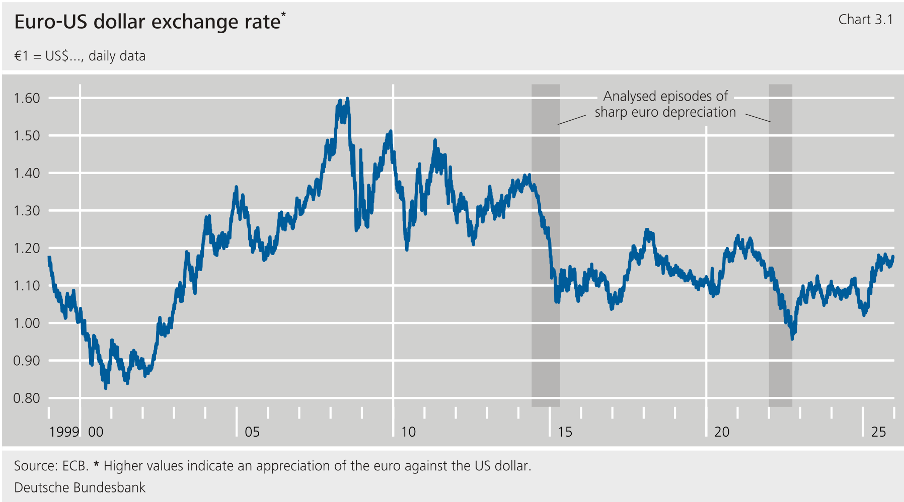
The euro-US dollar exchange rate has fluctuated considerably over time (Chart 3.1). The euro is currently trading at around US$1.17 – close to its price when the currency was introduced in 1999. It fell to a low of just over US$0.83 in the year immediately after its launch. This was followed by an eight-year period until early 2008 in which it doubled its value against the US dollar to US$1.59. The euro-US dollar exchange rate has also changed significantly at times during shorter time periods. For example, the euro lost around a quarter of its value against the US dollar in the three quarters from mid-2014 and shed around a fifth after January 2022 (grey shaded areas). But what are the causes of such fluctuations?

A glance at events triggering an immediate sharp appreciation or depreciation of the euro provides an initial indication of possible causes. Financial market prices such as the euro-US dollar exchange rate reflect the expectations of market participants. Market prices contain publicly available information and rate changes are attributable to new information that was previously not known. Particularly in the liquid euro-US dollar foreign exchange market, financial market participants respond immediately to new information that is significant for market prices. These are the considerations underlying event studies in economic and financial analyses: if price movements in response to identified events are examined in a time window that is narrow enough to exclude other potential determinants, sharp movements can be causally attributed to the event in question.

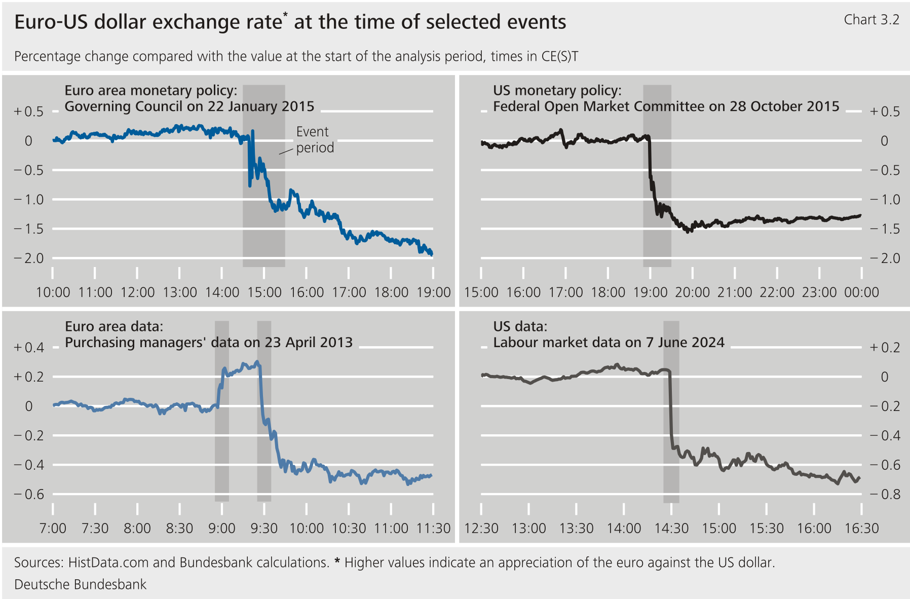
Examples of such events are monetary policy announcements. The upper left-hand panel in Chart 3.2 illustrates the performance of the euro-US dollar exchange rate on 22 January 2015. ECB President Draghi announced at the time that the Governing Council had decided to implement the asset purchase programme (APP). Because the scope of the programme exceeded market expectations, the euro depreciated by around 1 % within a narrow time frame surrounding the press conference of the ECB Governing Council (grey shaded area). 4 A similar movement took place on 28 October 2015, as illustrated in the upper right-hand panel. At around 19:00 Central European Time, the Fed’s Open Market Committee announced its monetary policy decision: its policy rate would remain unchanged as expected. However, it became clear in the course of the communication that an interest rate hike was closer than market participants had expected. The exchange rate, which had barely moved during the afternoon, responded immediately and the euro lost more than 1 % of its value against the US dollar within a few minutes.

The exchange rate sometimes also responds significantly to the publication of macroeconomic indicators. The lower left-hand panel of Chart 3.2 illustrates the development of the exchange rate on the morning of 23 April 2013 with two recognisable leaps. These are attributable to the publication of the purchasing managers’ index figures in the euro area. 5 Finally, in the lower right-hand panel of the chart the euro depreciated following the announcement of surprisingly strong US labour market data. Here as well, the sharp immediate reaction suggests that this event was the cause of the exchange rate movement.

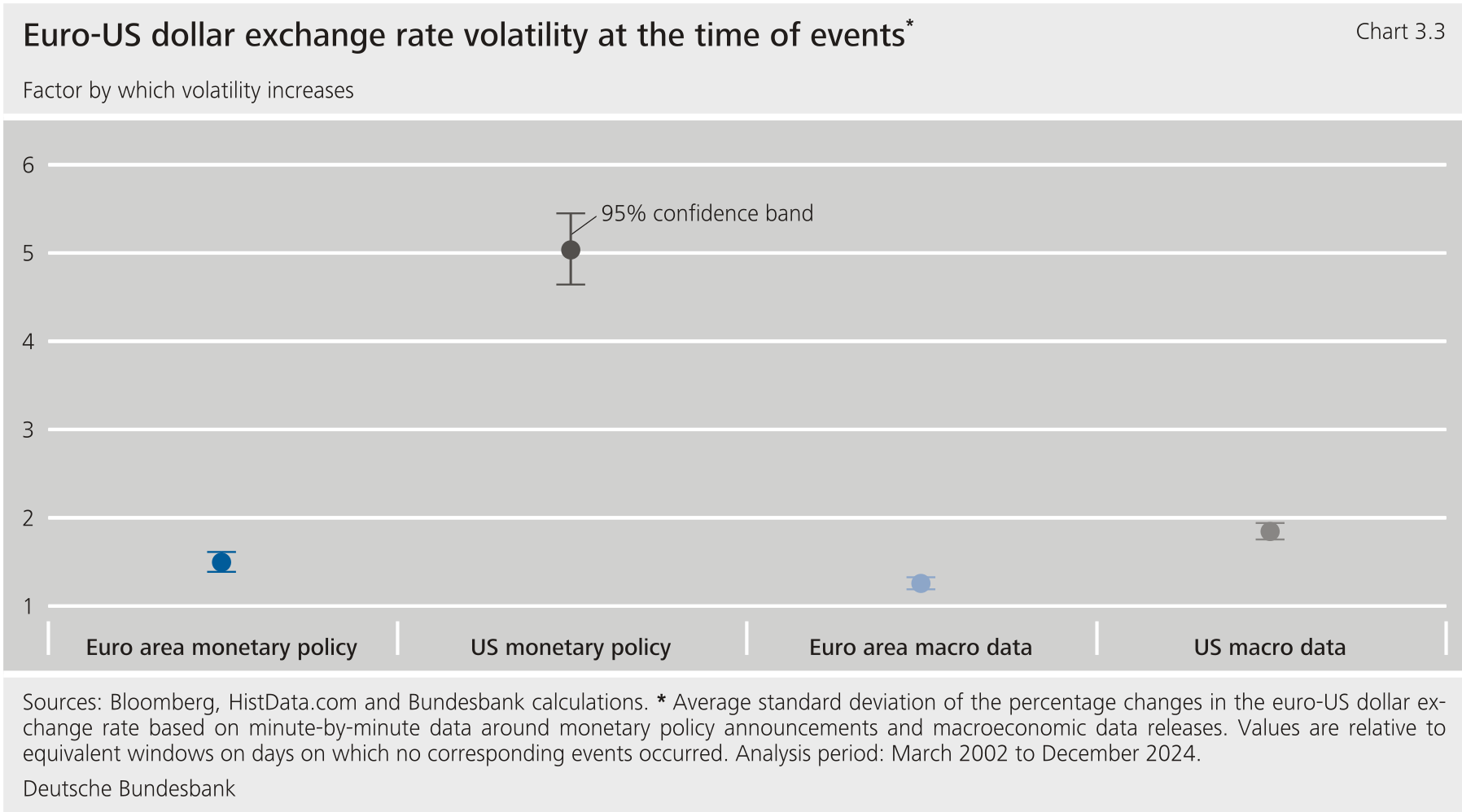
Such events, particularly Fed monetary policy announcements, are in fact a systematic source of exchange rate fluctuations. The examples illustrated above are not isolated cases. In order to quantify how influential events in a predefined category are, it is possible to calculate how much the exchange rate fluctuates on average in narrow time frames surrounding these events (Chart 3.3). 6 Doing so reveals that the volatility at the time of monetary policy announcements of the ECB Governing Council is around 50 % higher than in equivalent time periods without news about monetary policy in the euro area (dark blue). 7 Monetary policy news from the Federal Open Market Committee even increases volatility by a factor of five (dark grey). This indicates that market participants consider information about the Fed’s monetary policy stance to be particularly relevant for the euro-US dollar exchange rate. The difference from European monetary policy could be attributable to the fact that market participants attach greater weight to announcements concerning US monetary policy or that they were more frequently surprised by Fed announcements in the period under review. 8 The fact that news from the United States increases the volatility of the exchange rate more than news from the euro area also applies to macroeconomic data publications. The publication of key figures in the euro area only causes the exchange rate to fluctuate around 20 % more than it does normally (light blue). 9 By contrast, data publications in the United States increase volatility by almost 100 %. 10

Econometric analyses are needed to determine economic drivers of the exchange rate and quantify them over longer time periods. As outlined above, event studies show that news about monetary policy and the economy triggers sharp exchange rate movements. However, such studies only have limited informative content in that they are restricted to very short time periods surrounding the respective events. They therefore do not permit any conclusions to be drawn regarding the ups and downs of the euro over longer periods, for which econometric models are needed.

3 From event studies to determinants of the exchange rate over time

Econometric models allow the information from event studies to be transferred to longer time periods. Vector autoregressive (VAR) models are used to determine statistically how multiple variables typically move in relation to each other over days, weeks or months. However, additional information needs to be drawn on in order to be able to make statements about the different drivers of the financial variables. The event studies addressed above can be one source of such information. The responses to events measured with high-frequency data can be used to isolate the impact of individual determinants on the variables in the model (see the supplementary information entitled “A financial market model based on event studies (proxy VAR).” 11

Supplementary information

A financial market model based on event studies (proxy VAR)

A vector autoregressive (VAR) model is a statistical time series model consisting of a set of variables that are related to one another over time. Each of the $ n $ model variables is regressed on lagged values of all the variables in the model, mathematically expressed as

$$ y_t = c + B_1y_{t-1} + B_2y_{t-2} + ... + B_py_{t-p}+u_t $$

where $ y_t $ and $ c $ are $ (n \times 1) $ vectors of the endogenous model variables and constants, respectively, and $ p $ is the number of lags included. The $ (n \times n) $ matrices $ B i $ (where $ i = 1,...,p $) contain the estimated regression coefficients, which indicate how the variables interact with one another over time. Lastly, $ u_t $ is an $ (n \times 1) $ vector of error terms.

A total of ten financial market variables at a daily frequency are fed into the model estimated here: 1 Yields of German and US two and ten-year government bonds as well as (in logarithmic form) the EuroStoxx 50 equity index, the S&P 500, the VIX (a measure of S&P 500 volatility derived from option prices), the oil price in US dollars (Brent Crude Future), the gold price in US dollars and lastly the euro-US dollar exchange rate. 2 The model is estimated using Bayesian methods with $ p = 21 $ lags for the period from March 2002 to December 2025. 3

In order to be able to make statements about the economic determinants of financial market developments, the estimated residuals of the model need to be decomposed into their impulses (“shocks”). The estimated error terms $ \hat u_t $ – that is, the model residuals – are deviations of the observed data from the values predicted by the model. Viewed in isolation, though, they do not permit any conclusions regarding the impulses behind them, which are referred to as structural shocks. This is mathematically due to the fact that the residuals are correlated with each other. To instead identify the underlying determinants, it is interesting to see what happens if only one of these influencing factors arises and all the others remain untouched. This is made possible by converting the correlated residuals into uncorrelated shocks. While the residuals, then, comprise a mixture of shocks, the latter can be interpreted causally as distinct economic, structural determinants that in sum add up to the estimated error term.

Shocks are identified in a proxy VAR by means of instrumental variables – in this case, six of them. Instrumental variables are used here that correspond to the changes in financial market prices around certain events. These are measured in such narrow windows (such as five minutes before, to ten minutes after a given event) that the observed price changes are assumed to be almost exclusively attributable to those particular events. A causal relationship is thus assumed within the window. This information is transposed into the model by regressing the model residuals on the instrumental variables via a least squares estimation. The coefficients are then fed into the calculation of the impulse response functions. The individual instruments are assigned to their shocks by maximising the correlation of the shocks with their respective instruments. 4

Changes in interest rates around announcements by the ECB Governing Council and the Federal Reserve’s Open Market Committee are used to identify monetary policy shocks in the euro area and the United States. Not only the reactions of money market rates are measured, but also changes in the yields of longer-dated government bonds. This is done so that forward guidance and the effects of asset purchase programmes (quantitative easing), such as when short-term interest rates are at the zero lower bound, are covered. 5 Lastly, allowance is made for the fact that direct changes in interest rates can happen not just for reasons purely related to monetary policy, but also due to information effects. 6

Interest rate, equity price and exchange rate movements around the release of macroeconomic data serve as instruments for shocks to aggregate demand. If a data release triggers the impression that aggregate demand is higher than previously expected, equity prices and yields should surge upwards and cause the domestic currency to appreciate. Events comprising such a combination of financial market reactions thus form the basis for instruments for shocks affecting demand. However, a particular feature of the analysis lies in the fact that it does not simply take into account all data releases displaying such patterns. Instead, the events are each selected by means of an algorithm in such a way that, applied at a monthly frequency as instruments in VAR models, they also have macroeconomic effects that are associated with changes in demand: output and prices must rise or fall in synchronisation. 7

Energy price shocks are instrumented with oil price changes around the time of OPEC announcements and important news concerning supply in the European gas market. They therefore capture supply-side changes in energy markets. If, for instance, the oil price rises in direct response to announcements by OPEC (Organization of the Petroleum Exporting Countries), this is attributed to an expected reduction in output. 8 To also capture the gas market – a market that is particularly important for Europe – the exercise incorporates supply-side events that have elicited a strong response by the gas price. 9

Lastly, major changes in the VIX around selected events are used as an instrument for shocks to the risk appetite of international investors. The VIX measures the implied stock market volatility of the S&P 500 and thus expresses uncertainty surrounding the future performance of equity markets. If the VIX rises sharply in response to clearly identifiable events, this indicates a risk-off movement in which investors switch from risky to safe forms of investment. 10 In keeping with the literature, sharp movements of the VIX in response to such events are therefore drawn on to capture changes in risk appetite. 11

Footnotes

The model used here is a slightly modified version of the variant estimated in Karau (2026). The historical decompositions of the euro-US dollar exchange rate illustrated in the main article are based on a model in levels, as in Pinter et al. (2025). Results of a model estimation in which the variables are fed into the model in first differences yield similar findings.
All the variables, including the European ones, are measured at closing prices in the United States. For the most part, then, they relate to 22:00 Central European Time (CET), which is when the US financial markets close. This is important insofar as all the individual series thus comprise the same level of information. The prices of European financial market variables at 22:00 CET are approximated by adding to their closing prices in European trading (at 17:30 CET) the price change between 17:30 and 22:00 based on high-frequency futures data from the EUREX futures exchange.
Taking into account weekends, when no trading takes place, 21 lags is equivalent to around a month of observations. The estimation period starts in March 2002, as there are no high-frequency data available prior to this for calculating European variables at US closing prices; see footnote 2.
This represents an extension of the method developed in Piffer and Podstawski (2018) that is in turn based on the approach presented in Mertens and Ravn (2013). Unlike Piffer and Podstawski (2018), a precisely defined structural model is found for all six shocks, rather than many possible structural models for two shocks. This takes place mathematically by selecting the rotation of orthonormal matrices in such a way that the ratio of the sum of squared entries on the off-diagonal to on-diagonal entries is minimised in the matrix of correlation coefficients of instruments and shocks; see Karau (2026).
To consolidate the interest rates of government bonds of different maturities into a single measure, the first principal component of numerous changes in interest rates with maturities of one, three and six months and one, two and ten years is used. This principal component most strongly maps changes in the one to two-year segment that is frequently associated with forward guidance.
This is because if financial market participants believe that the central bank possesses information about future economic developments that was previously unknown to them and was therefore not already priced in, the observed market response might also be attributable to such information, rather than to the actual monetary policy tightening; see Nakamura and Steinsson (2018), Cieslak and Schrimpf (2019), Franz (2020), Miranda-Agrippino and Ricco (2021) and Kerssenfischer (2022). In such a case, positive interest rate surprises would be associated with rising equity prices, in contrast to an actual contractionary monetary policy shock. Accordingly, this exercise excludes the information effects, as in the literature, by only drawing on those interest rate surprises for determining contractionary monetary policy shocks that are associated with falling equity prices (see Jarociński and Karadi (2020)) and an appreciation of the euro.
According to the method developed in Alessandri et al. (2023), this is done by feeding the shocks identified in the daily model cumulatively as instrumental variables into a monthly VAR model. The events are then selected by means of an algorithm that ensures that industrial output and consumer prices rise in the monthly model; see Karau (2026).
Based on 90 of the OPEC announcements as of March 2002 used in Känzig (2021). In order also to filter out possible information effects here (from the perspective of market participants, OPEC announcements could also include assessments by OPEC regarding future demand for oil), the same approach is followed as in Degasperi (2023): Only those changes in oil prices to which the S&P 500 equity index responds with the opposite sign are used.
The 26 events in Alessandri and Gazzani (2024) are used for this. Many of these are connected to Russia’s war of aggression against Ukraine. For a similar analysis of the exchange rate effects of such gas price shocks during the Ukraine war, see Deutsche Bundesbank (2022).
As well as increased uncertainty about the future course of the economy (see Bloom (2014)), in economic models this can, for instance, reflect changes in investor confidence (Angeletos et al. (2018)) or a rise in risk aversion among investors (Campbell et al. (2020)).
The events identified via a narrative approach in Gazzani et al. (2024) are used for this. These are selected so that in addition to a rise in the VIX, gold prices also pick up, while the oil price falls.

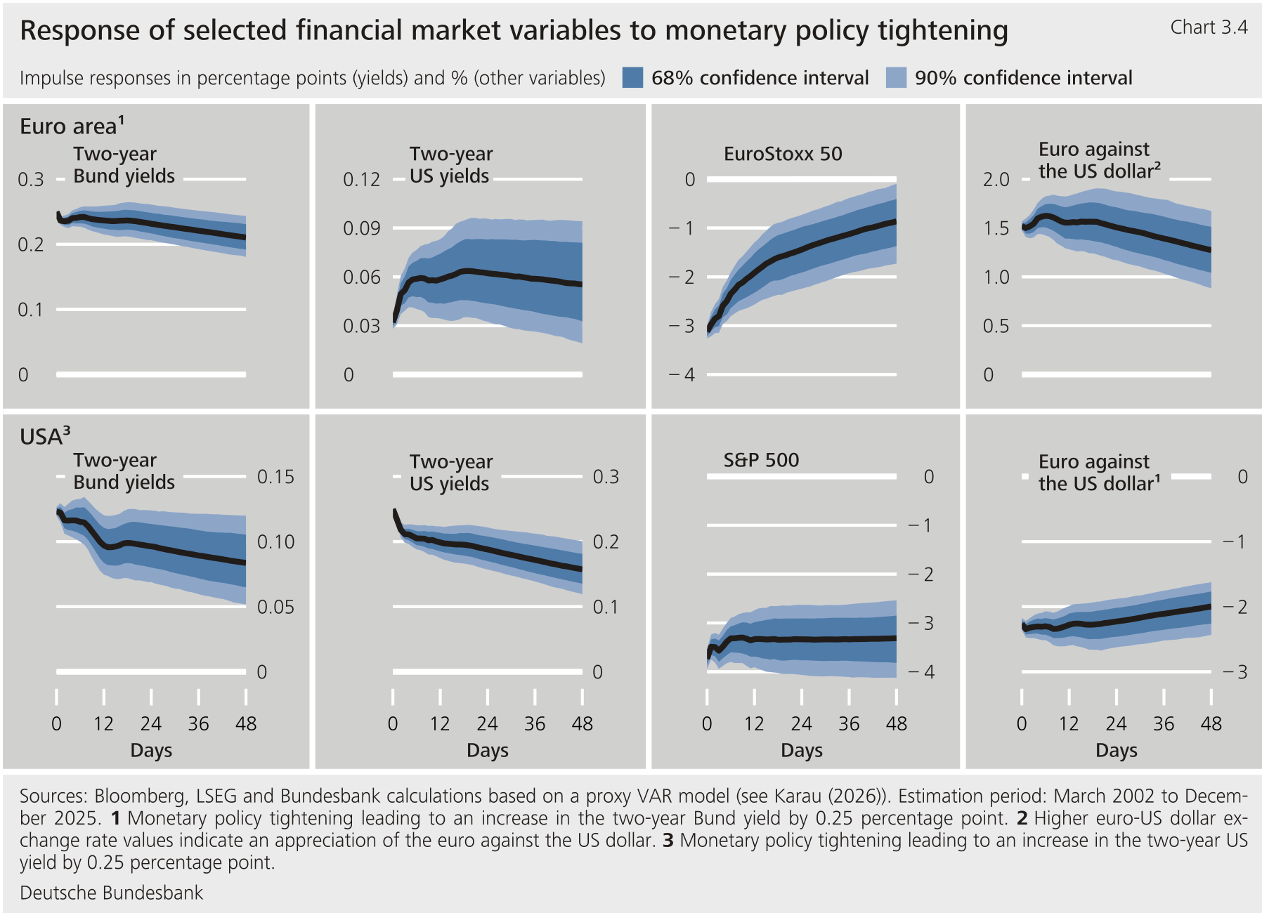
One such approach is used here to determine the causal effects of individual drivers of the euro-US dollar exchange rate in a financial market model. In order, for instance, to assess the impact of monetary policy, it is possible to measure how money market rates and yields on bonds in tight time windows react to monetary policy announcements. Once incorporated into the model, the effects can then be calculated over time. Chart 3.4 illustrates an example of this and comprises two sequences of impulse response functions. These provide information about how four out of a total of ten financial market prices contained in the model respond over time if monetary policy in the euro area (above) or in the United States (below) is unexpectedly tightened.

Monetary policy impulses from the United States exert a particularly strong impact on the euro-US dollar exchange rate (Chart 3.4). The top part of the chart examines a monetary policy impulse from the euro area that causes two-year German government bonds (Bunds) to rise by 25 basis points. European equity market valuations immediately fall by around 3 % in response before gradually recovering in the following days. US yields also rise, but only by around six basis points, causing the interest rate differential to therefore widen by around 20 basis points in favour of the euro area. Because this relative rise in the interest rate attracts capital, it also causes the euro to appreciate and immediately gain around 1.5 % in value against the US dollar. 12 If, by contrast, US monetary policy is tightened as in the lower panel of the chart and US interest rates rise by 25 basis points, domestic equity valuations likewise fall. A monetary policy shock from the United States has a greater impact on two-year Bunds than its counterpart from the euro area on the United States. The relative rise in the interest rate is correspondingly lower in the United States at just over ten basis points. And yet the exchange rate still responds more sharply: the euro depreciates by more than 2 % against the US dollar. This is at first glance surprising as it initially suggests that the amount of change of the interest rate differential is the decisive factor influencing the strength of the exchange rate’s reaction. However, it is well documented in the economic literature that, as well as the interest rate differential, risk premiums also play an important role in determining exchange rates 13 which are also influenced by monetary policy. 14

This model approach can be used to track down further drivers of the euro‑US dollar exchange rate alongside monetary policy changes. As with monetary policy impulses, they are identified by means of high-frequency data in the VAR model (see the supplementary information entitled “A financial market model based on event studies (proxy VAR)”). The financial market reactions to publications of macroeconomic data described above are used to assess the impact of changes in aggregate demand. In order to understand increased risk aversion on the financial markets, changes to implied stock market volatility (VIX) are measured at the time of selected events when investors shift their assets from risky to safe investments. And finally, oil price changes are measured around news regarding the supply of oil and gas.

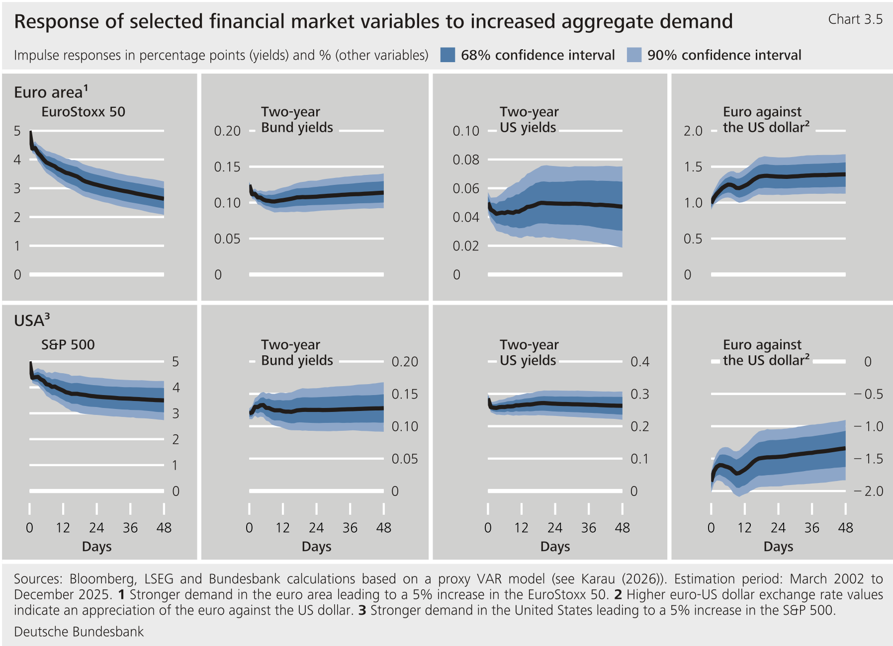
The euro appreciates when economic activity in the euro area increases and depreciates when activity in the United States picks up (Chart 3.5). In the case of a boost in demand from the euro area (top) that immediately triggers a 5 % surge in the EuroStoxx 50, two-year Bunds rise by just over ten basis points. US yields also react positively, but the effect is smaller. The interest rate differential accordingly widens in favour of the euro area, causing the euro to appreciate by more than 1 % against the US dollar. A boost in demand from the United States (lower panel) conversely leads to a persistent depreciation of the euro, also due to the fact that yields rise more on the other side of the Atlantic than on this side.

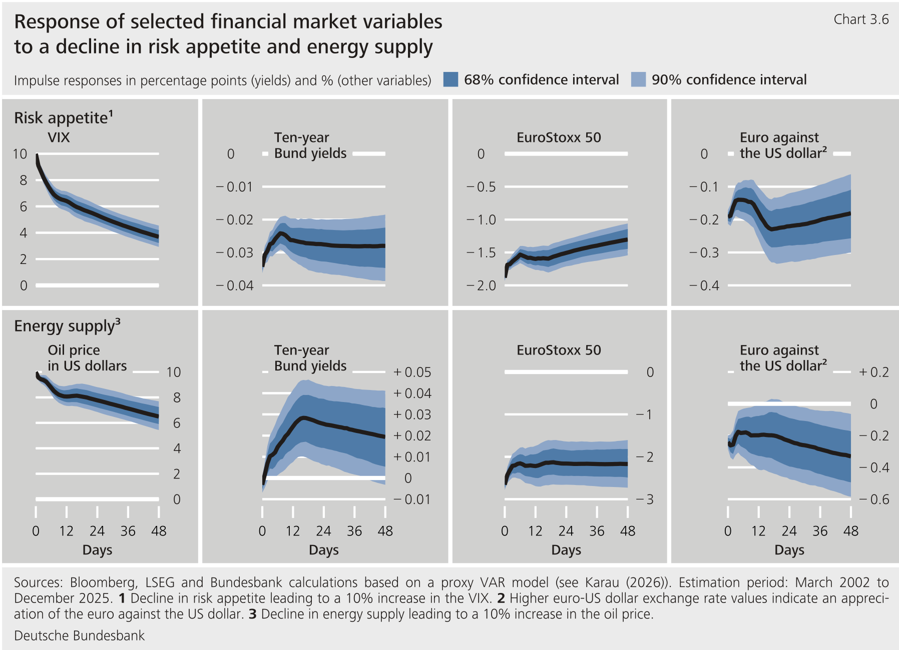
The euro is weakened by a decline in global risk appetite and a shortage of supply on the energy markets (Chart 3.6). A 10 % rise in the VIX induced by a fall in risk appetite (upper panel) leads to a portfolio shift from risky assets such as equities to safer bonds, the yields of which decline by several basis points. The value of the euro also decreases by around 0.2 % compared with the US dollar, which is considered at least historically to be a safe haven in times of growing risk aversion in financial markets. 15 A 10 % rise in the oil price (lower panel) leads to only minor changes to yields in the model but a prolonged decline in European equity prices of more than 2 %. The euro loses just over 0.2 % in value against the US dollar. 16

4 Which factors were responsible for the depreciation of the euro against the US dollar in 2014‑15 and 2022?

After assessing how the individual factors impact financial market variables over time, their relative importance for observed exchange rate developments can be quantified. Simply eyeballing the estimated impulse response functions can sometimes already provide an indication as to which determinants were particularly important in a given episode. 17 Generally, however, the impulses of many of the factors will overlap and their contributions will also change over time. Having said this, the movements of individual financial market variables can also be systematically decomposed in the model into the contributions of all identified drivers. This accordingly sheds light on their relative importance.

One episode of particular interest is the sharp depreciation of the euro against the US dollar in 2014‑15. At this time the euro lost around a quarter of its value against the US dollar over nine months. This period is especially interesting from a monetary policy perspective, as interest rates on both sides of the Atlantic were close to zero, while expected paths of monetary policy pointed in clearly different directions: Whereas market participants speculated on when the Fed would introduce a tightening cycle, the signs in the Eurosystem were set towards a further easing of monetary policy.

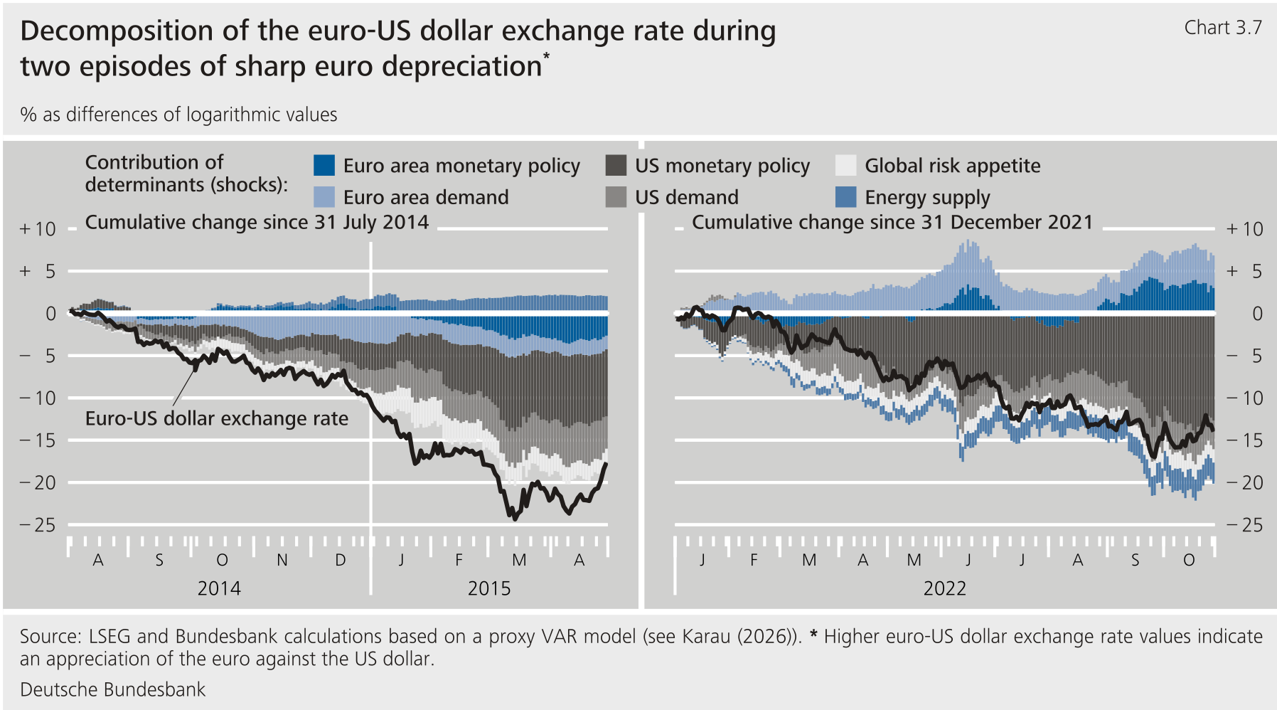
A historical decomposition within the scope of the VAR model used reveals that the development was significantly driven by Fed monetary policy throughout the entire depreciation period (Chart 3.7, left panel). The chart illustrates the development of the euro-US dollar exchange rate since the summer of 2014 (black line) together with the contributions of the individual influencing factors (coloured bars). 18 According to the model, the greatest contribution to the depreciation of the euro was made by US monetary policy (dark grey). This is striking in as much as the Fed did not hike its monetary policy rate at all until the end of 2015. The model nevertheless captures a noticeable swing from an expansionary zero interest policy to a tightening, expressed by the Fed winding down its asset purchases and market participants increasingly expecting interest rate hikes to be imminent.

The impact of the asset purchase programme of the Eurosystem is also clearly visible. As mentioned in the context of Chart 3.2, the euro depreciated immediately following the announcement of the APP. Chart 3.7 now reveals that the expansionary stance of the Eurosystem’s monetary policy contributed up to around three percentage points to the euro’s depreciation since mid-January 2015 (dark blue). The impact of the non-standard monetary policy on the exchange rate impact was thus roughly similar to that of an interest rate policy reducing two-year yields by 50 basis points. Altogether, however, the impact of the APP on the exchange rate probably remained lower in the period under review here than that of US monetary policy. 19 Weaker aggregate demand in the euro area (light blue) and stronger aggregate demand in the United States (light grey) likewise exerted downward pressure on the euro, as did a downturn in global risk appetite (white). The only factor supporting the euro according to the model estimation was more favourable conditions on the energy market that at that time weighed strongly on the oil price (medium blue).

US monetary policy likewise accounted for a large share of the sharp depreciation of the euro in 2022 – together with the disruption on the energy market due to the Russian war of aggression against Ukraine (Chart 3.7, right panel). The euro depreciated by just over 15 % against the US dollar in the course of 2022. According to the model estimation, this was likewise largely attributable to market participants increasingly pricing in an imminent tightening of US monetary policy. However, the euro was also adversely affected by rising energy prices due to the Russian war of aggression against Ukraine. Together with a decline in global risk appetite, these forces contributed several percentage points to the depreciation of the euro. 20 The exchange rate was supported by expectations among investors that interest rates would also rise in the euro area, and by the brightening of the economic outlook here somewhat compared with the start of 2022.

5 Concluding thoughts and outlook

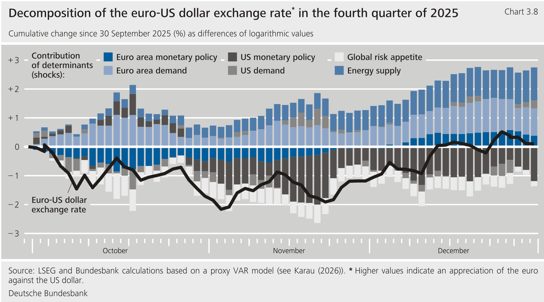
The method presented here of a proxy VAR model with financial market variables permits almost real-time conclusions to be drawn about determinants of exchange rate movements, thereby also providing an impression of general economic driving forces. The interplay of different financial market prices with the event studies used here can help to assess current dynamics in a timely manner. For example, although there was barely any change on balance in the euro-US dollar exchange rate in the fourth quarter of 2025, a decomposition of the exchange rate in the model reveals that market participants assessed the economic outlook in the euro area more positively at the end of the year than previously (Chart 3.8). Moreover, the euro was supported by the falling oil price. Meanwhile, changing assessments about how far the Federal Reserve will ease its monetary policy determined the evolution of the exchange rate. On the other hand, fewer impulses for the exchange rate came from the euro area’s monetary policy at the end of 2025 as the impression became increasingly established among market participants that the rate-cutting cycle in the euro area had come to an end.

This article is based on data available up to 31 December 2025, 22:00.

List of references

Alessandri, P. and A. Gazzani (2024), Natural gas and the macroeconomy: Not all energy shocks are alike, Journal of Monetary Economics, Vol. 151, 103749.

Alessandri, P., A. Gazzani and A. Vicondoa (2023), Are the Effects of Uncertainty Shocks Big or Small?, European Economic Review, Vol. 158, 103745.

Alessandri, P. and H. Mumtaz (2019), Financial Regime and Uncertainty Shocks, Journal of Monetary Economics, Vol. 101, pp. 31‑46.

Angeletos, G.-M., F. Collard and H. Dellas (2018), Quantifying Confidence, Econometrica, Vol. 86(5), pp. 1689‑1726.

Avdjiev, S., V. Bruno, C. Koch and H. S. Shin (2019), The Dollar Exchange Rate as a Global Risk Factor, IMF Economic Review, Vol. 67(1), pp. 151‑173.

Bank for International Settlements (2025), Triennial Central Bank Survey of foreign exchange and Over-the-counter (OTC) derivatives markets in 2025.

Baumeister, C. and J. D. Hamilton (2019), Structural Interpretation of Vector Autoregressions with Incomplete Identification: Revisiting the Role of Oil Supply and Demand Shocks, The American Economic Review, Vol. 109(5), pp. 1873‑1910.

Bauer, M. D. and E. T. Swanson (2023), A Reassessment of Monetary Policy Surprises and High-Frequency Identification, NBER Macroeconomics Annual, Vol. 37, pp. 87–155.

Bloom, N. (2014), Fluctuations in Uncertainty, Journal of Economic Perspectives, Vol. 28(2), pp. 153‑176.

Boehm, C. E. and T. N. Kroner (2025), The U.S., Economic News, and the Global Financial Cycle, The Review of Economic Studies, Vol. 93(1), pp. 215–249.

Bouakez, H. and M. Normandin (2010), Fluctuations in the Foreign Exchange Market: How Important are Monetary Policy Shocks?, Journal of International Economics, Vol. 81(1), pp. 139‑153.

Bruno, V. and H. S. Shin (2015), Capital Flows and the Risk-Taking Channel of Monetary Policy, Journal of Monetary Economics, Vol. 71, pp. 119–132.

Campbell, J. Y., C. Pflueger and L. M. Viceira (2020), Macroeconomic Drivers of Bond and Equity Risks, Journal of Political Economy, Vol. 128(8), pp. 3148‑3185.

Cieslak, A. and A. Schrimpf (2019), Non-monetary News in Central Bank Communication, Journal of International Economics, Vol. 118(C), pp. 293–315.

Degasperi, R. (2023), Identification of Expectational Shocks in the Oil Market Using OPEC Announcements, mimeo.

Degasperi, R., S. S. Hong and G. Ricco (2024), The Global Transmission of U.S. Monetary Policy, Banca d’Italia, Temi di discussione (Economic Working Papers), No 1466.

Deutsche Bundesbank (2025a), Risk appetite in financial markets and monetary policy, Monthly Report, January 2025.

Deutsche Bundesbank (2025b), Financial markets, Monthly Report, February 2025.

Deutsche Bundesbank (2025c), Financial market environment, Monthly Report, May 2025.

Deutsche Bundesbank (2022), Rise in energy prices, the exchange rate of the euro and Germany’s price competitiveness, Monthly Report, December 2022, pp. 45‑54.

Deutsche Bundesbank (2020), The impact of monetary policy on the euro’s exchange rate, Monthly Report, September 2020, pp. 19‑51.

Deutsche Bundesbank (2017), The Eurosystem’s bond purchases and the exchange rate of the euro, Monthly Report, January 2017, pp. 13‑39.

Deutsche Bundesbank (2014), Exchange rates and financial stress, Monthly Report, July 2014, pp. 15‑28.

Dornbusch, R. (1976), Expectations and Exchange Rate Dynamics, The Journal of Political Economy, Vol. 84(6), pp. 1161‑1176.

Eichenbaum, M. and C. L. Evans (1995), Some Empirical Evidence on the Effects of Shocks to Monetary Policy on Exchange Rates, The Quarterly Journal of Economics, Vol. 110(4), pp. 975–1009.

Engel, C. (2016), Exchange Rates, Interest Rates, and the Risk Premium, American Economic Review, Vol. 106(2), pp. 436‑474.

Fama, E. F. (1984), Forward and Spot Exchange Rates, Journal of Monetary Economics, Vol. 14(3), pp. 319‑338.

Forbes, K. J., I. Hjortsoe and T. Nenova (2020), International Evidence on Shock-Dependent Exchange Rate Pass-Through, IMF Economic Review, Vol. 68(4), pp. 721‑763.

Franz, T. (2020), Central bank information shocks and exchange rates, Deutsche Bundesbank Discussion Paper No 13/2020, March 2020.

Gazzani, A., F. Venditti and G. Veronese (2024), Oil price shocks in real time, Journal of Monetary Economics, Vol. 144, 103547.

Gertler, M. and P. Karadi (2015), Monetary Policy Surprises, Credit Costs, and Economic Activity, American Economic Journal: Macroeconomics, Vol. 7(1), pp. 44–76.

Georgiadis, G., G. J. Müller and B. Schumann (2024), Global risk and the dollar, Journal of Monetary Economics, Vol. 144, 103549.

Georgiadis, G., G. J. Müller and B. Schumann (2023), Dollar Trinity and the Global Financial Cycle, CEPR Discussion Paper, No. 18427.

Gopinath, G., E. Boz, C. Casas, F. J. Díez, P.O. Gourinchas and M. Plagborg-Møller (2020), Dominant Currency Paradigm, American Economic Review, Vol. 110(3), pp. 677‑719.

Gopinath, G. and J. C. Stein (2021), Banking, Trade, and the Making of a Dominant Currency, The Quarterly Journal of Economics, Vol. 136(2), pp. 783–830.

Ha, J., M. Stocker and H. Yilmazkuday (2019), Inflation and Exchange Rate Pass-Through, Journal of International Money and Finance, Vol. 105, 102187.

Heinlein, R. and H.-M. Krolzig (2012), Effects of Monetary Policy on the US Dollar/UK Pound Exchange Rate: Is There a “Delayed Overshooting Puzzle”?, Review of International Economics, Vol. 20(3), pp. 443‑467.

Jarociński, M. and P. Karadi (2020), Deconstructing Monetary Policy Surprises – The Role of Information Shocks, American Economic Journal: Macroeconomics, Vol. 12(2), pp. 1–43.

Juvenal, L. and I. Petrella (2015), Speculation in the Oil Market, Journal of Applied Econometrics, Vol. 30(4), pp. 621‑649.

Känzig, D. (2021), The Macroeconomic Effects of Oil Supply News: Evidence from OPEC Announcements, American Economic Review, Vol. 111(4), pp. 1092–1125.

Karau, S. (2026), Macro Shocks in Real Time, mimeo.

Karau, S. (2024), Relative Monetary Policy and Exchange Rates, Deutsche Bundesbank Discussion Paper, No 40/2024.

Kerssenfischer, M. (2022), Information effects of euro area monetary policy, Economics Letters, 216, 110570.

Kilian, L. (2009), Not All Oil Price Shocks Are Alike: Disentangling Demand and Supply Shocks in the Crude Oil Market, American Economic Review, Vol. 99(3), pp. 1053–1069.

Kilian, L. and C. Park (2009), The Impact of Oil Price Shocks on the U.S. Stock Market, International Economic Review, Vol. 50(4), pp. 1267‑1287.

Liao, W., J. Ma and C. Zhang (2023), Identifying Exchange Rate Effects and Spillovers of U.S. Monetary Policy Shocks in the Presence of Time-Varying Instrument Relevance, Journal of Applied Econometrics, Vol. 38(7), pp. 989‑1006.

McLeay, M. and S. Tenreyro (2026), Dollar Dominance and the Transmission of Monetary Policy, The Quarterly Journal of Economics, Vol. 141(1), pp. 605–666.

Mertens, K. and M. O. Ravn (2013), The Dynamic Effects of Personal and Corporate Income Tax Changes in the United States, American Economic Review, 103(4), pp. 1212‑1247.

Miranda-Agrippino, S. and T. Nenova (2022), A Tale of Two Global Monetary Policies, Journal of International Economics, 103606.

Miranda-Agrippino, S. and H. Rey (2020), U. S. Monetary Policy and the Global Financial Cycle, The Review of Economic Studies, Vol. 87(6), pp. 2754‑2776.

Miranda-Agrippino, S. and G. Ricco (2021), The Transmission of Monetary Policy Shocks, American Economic Journal: Macroeconomics, Vol. 13(3), pp. 74–107.

Nakamura, E. and J. Steinsson (2018), High-Frequency Identification of Monetary Non-Neutrality: The Information Effect, The Quarterly Journal of Economics, 133(3):12831330.

Ortega, E. and C. Osbat (2020), Exchange Rate Pass-Through in the Euro Area and EU Countries, ECB Occasional Paper Series, No 241.

Peersman, G. and I. Van Robays (2009), Oil and the Euro Area Economy, Economic Policy, Vol. 24(60), pp. 603‑651.

Piffer, M. and M. Podstawski (2018), Identifying Uncertainty Shocks Using the Price of Gold, The Economic Journal, Vol. 128(616), pp. 3266‑3284.

Pinter, G., F. Smets and S. Üslü (2025), Market whiplash after the 2025 tariff shock: An event-targeted VAR approach, BIS Working Papers, No 1282.

Rey, H. (2013), Dilemma not Trilemma: The Global Financial Cycle and Monetary Policy Independence, in: Federal Reserve Bank of Kansas City (eds.): Global Dimensions of Unconventional Monetary Policy, Jackson Hole Economic Policy Symposium Proceedings, pp. 285‑333.

Rüth, S. K. (2020), Shifts in monetary policy and exchange rate dynamics: Is Dornbusch’s overshooting hypothesis intact, after all?, Journal of International Economics, Volume 126,103344.

Scholl, A. and H. Uhlig (2008), New Evidence on the Puzzles: Results from Agnostic Identification on Monetary Policy and Exchange Rates, Journal of International Economics, Vol. 76(1), pp. 1–13.

Stock, J. H. and M. W. Watson (2018), Identification and Estimation of Dynamic Causal Effects in Macroeconomics Using External Instruments, The Economic Journal, Vol. 128(610), pp. 917–948.