Non-final working translation 

The global economy is navigating a period of prolonged geopolitical tensions. Geopolitical and economic policy uncertainty has risen significantly in recent years (see Chart 1.1.1, left-hand side). 1 At the same time, fragmentation of the global economy has risen to historically high levels. Strains in global supply chains remain elevated (see Chart 1.1.1, centre and right-hand side). 2 Adding to these challenges, hybrid threats and cyber risks are increasingly jeopardising the stability of the financial system (see Section 1.2). These developments not only heighten overall uncertainty but also increase the likelihood of further adverse supply shocks. As a result, they could dampen economic activity, intensify inflationary pressures and pose considerable adjustment challenges for firms. In addition, there is a heightened risk that financing conditions will suddenly tighten and asset prices fall. 3 The extent to which these dynamics affect individual economies and the stability of their financial systems depends on their specific vulnerabilities to these developments.

Geopolitical tensions are taking a particularly heavy toll on the German economy. By European standards, Germany has a high export ratio and is therefore particularly reliant on global economic activity and international trade dynamics (see Chart 1.1.2, left-hand side). At the same time, a comparatively large share of Germany’s gross value added stems from the manufacturing sector (see Chart 1.1.2, centre). This makes Germany particularly vulnerable to trade barriers, supply chain disruptions and energy and shocks to input prices. As a result, economic policy uncertainty has risen more sharply than in other countries. It remained at a high level during the reporting period and continues to hover close to historical highs (see Chart 1.1.2, right-hand side). 4 The high level of uncertainty could also weigh on investment and production decisions, making a sustained economic recovery more difficult. 5

The German economy has emerged from the recession, but downside risks remain high. After two years of economic contraction, real gross domestic product (GDP) posted a modest increase in 2025. The gradual recovery is proceeding in 2026. This development is expected to continue in 2027. Forecasts for economic growth over the reporting period were revised downwards significantly at times due to the impact of the conflict in Iran on commodity prices, real wages and general uncertainty. 6 However, the German economy has shown unexpected resilience so far. It is also benefiting from temporary one-off effects caused by the conflict in Iran, for example because firms in Asia are more heavily affected by supply chain disruptions. Firms are cautious in their response to economic and geopolitical uncertainty. While sentiment indicators in the manufacturing sector in Germany have improved recently on a broad basis, firms’ confidence remains subdued, both in absolute terms and in comparison with other European countries (see Chart 1.1.3). The model-based approach of the Financial Stability Frontier helps to assess the extent to which expected economic developments entail risks to financial stability (see the supplementary information entitled “The Financial Stability Frontier: model-implied assessment of macro-financial fragility in the euro area”). The approach does not currently signal financial fragility but shows that risks to financial stability remain elevated owing to the ongoing uncertainty surrounding the economic outlook.

Economic growth in 2026 will be largely driven by expansionary fiscal policy. Up to 2028, the cumulative fiscal contribution to growth is expected to be around 1.3 percentage points, driven in particular by higher defence expenditure. 7 However, the medium-term growth outlook and potential output will only improve on a sustained basis if fiscal resources are employed in such a way that they raise productivity. Otherwise, sovereign financing needs and the interest burden on households and firms will increase. This would weigh on the macro-financial environment in the long term, further limit fiscal space for future crises and amplify risks to financial stability (see Section 1.3). 8

Structural barriers are weighing on the growth outlook beyond the negative impact of recent supply shocks. The German economy is not only experiencing a period of cyclical weakness, but is also facing a far-reaching adjustment process. 9 Whilst industrial production has largely stabilised in many European economies following the pandemic-related slump, the downward trend in Germany, which has been ongoing since 2018, is continuing (see Chart 1.1.4). This indicates that structural burdens, in addition to cyclical factors, are constraining potential output. High energy costs, demographic ageing 10 , technological changes, increased competitive pressure, growing geoeconomic fragmentation and the high costs of doing business in Germany are dampening potential output and intensifying adjustment pressures (see Section 1.5). 11 At the same time, weak growth prospects and heightened uncertainty could weigh on investment. If investment remains sluggish in the long term, this could impair productivity growth and further dampen potential output. Greater diversification and regionalisation of supply chains could strengthen the resilience of the German economy to adverse external developments. However, such measures often come with higher costs and efficiency losses at first.

Lower growth potential could have a negative impact on the stability of the German financial system. Weaker corporate profitability and household income, diminished employment prospects and a higher burden on public finances could impair borrowers’ debt sustainability and raise default risks. At the same time, lower earnings expectations and weaker economic growth could put pressure on asset valuations. This heightens the risk of losses for banks and other financial intermediaries. 12

Structural reforms that strengthen growth and economic adaptability over the long-term would support financial stability. On the supply side, public investment in infrastructure, research and development and in accelerating the energy transition would bolster growth forces in the long term. Faster planning, approval and procurement procedures could also play a role here. A broader application of digital technologies and artificial intelligence could further boost productivity, especially among small and medium-sized enterprises. Expanding labour supply through greater incentives to participate in the labour market, skilled immigration, training and a higher effective retirement age could cushion demographic pressures. On the financing side, a more investment-friendly tax framework and better financing conditions for start-ups and scale-ups would promote private investment and business dynamism. At the European level, further deepening of the Single Market and better cross-border financing conditions could additionally play a role in facilitating the scaling and investments of European firms and thus strengthen the competitiveness of the European Union (EU). Overall, structural reforms could bring lasting improvements in profitability, employment, debt sustainability and competitiveness.

The downside risks to the macro-financial environment remain substantial. While the German economy has so far been unexpectedly robust and is benefiting in part from temporary competitive advantages, this is offset by persistent structural challenges and high economic policy uncertainty. According to the Deutsche Bundesbank’s growth-at-risk model, highly negative growth rates remained just as likely compared with the previous year (see Chart 1.1.5). 13 A further escalation of geopolitical conflicts, additional trade barriers or renewed disruptions to global supply chains could increase the downside risks to the economy. Recurring supply shocks also entail the risk of higher inflation volatility. They could have a negative impact on financing conditions and thus further amplify downside risks.

In addition to downside macro-financial risks, risks from cyberattacks and hybrid threats are becoming increasingly important. The ongoing digitalisation of the financial system and continued technological developments, such as those in the field of artificial intelligence (AI), are creating new operational vulnerabilities. These can be exploited in a targeted manner by malicious agents. In the context of heightened geopolitical tensions, particularly since the beginning of Russia’s war of aggression against Ukraine, state and state-affiliated actors are increasingly at risk. Cyberattacks can occur in isolation or in the context of hybrid threats. Hybrid threats aim to impair the functioning or legitimacy of states or institutions. They may include such methods as cyberattacks, sabotage, espionage, information manipulation or threats of military force. Hybrid threats are also characterised by a high degree of ambiguity, which often makes it difficult to clearly attribute them to a specific attacker. 14  

Advances in the field of AI are exacerbating technological asymmetries in cyber security, with AI models developing the ability to significantly increase the speed, scalability and complexity of cyberattacks. In recent years, the time span between a security vulnerability being disclosed or coming to light and this vulnerability being provably exploited has shortened drastically – from several weeks to a matter of hours (see Chart 1.2.1). At the same time, AI can also improve cyber resilience by, for example, accelerating anomaly detection, analysing vulnerabilities and automating responses. The limited availability of particularly advanced AI models (frontier models) can therefore amplify technological asymmetries. This holds true for attackers versus defenders as well as between jurisdictions, as the leading providers of AI models are located outside Europe. Macroprudential bodies and supervisory authorities have responded to this development, with the ESRB issuing a warning on systemic cyber risks resulting from frontier models, for example. 15

In view of heightened geopolitical tensions, the risk of hybrid threats has increased. The financial system can also become a target of hybrid attacks. For example, attackers can exploit cyber security deficiencies in order to specifically attack critical points in the technological infrastructure of the financial system, such as central third-party service providers (see Section 2.6). Fake news, which is often disseminated via social media, can also have a systemic effect via the trust channel. Financial institutions and financial market infrastructures need to further strengthen their resilience to these new and complex challenges. Cooperation between authorities and sectors as well as rapid, forward-looking and credible communication are key for supervision. This applies equally at the national, European and international levels. 

Fiscal vulnerabilities in the euro area have increased further over the past year. They stem from several mutually reinforcing factors: structurally rising spending needs, weak growth, higher debt servicing costs and recurring macroeconomic shocks. 16  The new European fiscal rules require sustainable spending and debt paths over the medium term. In an environment of weak growth, higher interest rates and structurally increasing fiscal burdens, compliance with these rules becomes more challenging. This is particularly true for Member States with already high debt ratios, but also for Germany, whose fiscal stance has become more expansionary on account of its additional scope for borrowing for defence and infrastructure expenditure. From 2025 to 2028, the EU fiscal rules allow for an exceptional increase in defence expenditure of up to 1.5% of GDP per year. 17 Furthermore, an exemption for energy-related measures will apply from 2026 to 2028. This would extend the annual budgetary scope in the period up to 2028 by up to an additional 0.3% of GDP. Deficits are thus likely to rise further in the coming years.

The European Commission’s long-term projections show a significant increase in the euro area debt ratio. 18  Should the policy stance remain unchanged, the European Commission reports that the euro area debt ratio will rise from 88% of GDP in 2025 to 105% in 2036. The projected debt path is thus 3 percentage points higher than in the Commission’s 2025 projections. In many European countries, debt ratios are still elevated or are expected to rise further. For the group of euro area countries with higher debt levels, the debt ratio is projected to reach around 140% of GDP (see Chart 1.3.1, left-hand side). Meanwhile, structural spending needs for defence, infrastructure, climate change adaptation and managing the consequences of demographic ageing are increasing. Both these factors reduce the fiscal space available to stabilise future macro-financial shocks. Negative supply shocks, in particular, may weigh on debt sustainability by dampening real growth and simultaneously prompting government support or relief measures, as was the case recently during the energy price shocks. Higher spending and potentially lower revenue then further increase the debt ratio.

Higher interest rates are feeding through to public finances with a lag, but their impact is being increasingly felt. Sovereign bond yields have risen significantly alongside the increase in interest rates following the coronavirus crisis (see Chart 1.3.1, right-hand side). Across much of the euro area, financing costs have returned to levels last seen before the low interest rate period of the 2010s. The long average maturity of government debt will initially cushion the direct effect of higher market interest rates. However, interest expenditure will gradually increase as debt is refinanced at higher interest rates. This is particularly relevant for countries with high debts, persistent primary deficits and weak growth. According to the European Commission, interest expenditure in more highly indebted countries could reach more than 5% of GDP by 2036 (see Chart 1.3.1, centre panel). 19 A sudden reassessment of fiscal risks in individual countries by market participants could drive risk premia up and pass through to the financing costs of enterprises and banks. 

In Germany, making full use of the available fiscal leeway will entail substantial fiscal consolidation needs going forward. The debt-to-GDP ratio already rose by 1.4 percentage points to 62.8% in 2025, and is expected to climb to around 70% in 2028, the Bundesbank’s forecast says. According to the forecast, the deficit ratio will rise to almost 5% over the same period. Fiscal policy is making extensive use of the additional borrowing capacity granted. This is likely to continue pushing the debt ratio up in the medium term too: European Commission projections point to a significant increase in the debt ratio to up to over 90% of GDP by the mid-2030s if policy remains unchanged (see Chart 1.3.2, left-hand side). It is true that Germany’s debt ratio and interest burden are still below average by European standards. However, even without limiting the scope for defence-related borrowing, the rising interest burdens (see Chart 1.3.2, right-hand side) and additional expenditure caused by the ageing of the population will create conflicts with the debt brake from 2028 onwards. The national borrowing limits do not yet ensure compliance with the European fiscal rules. Considerable further adjustments will be needed to achieve this. 

Elevated risks related to debt sustainability in the euro area could impair the stability of the German financial system through the sovereign-bank nexus and cross-border contagion effects. The sovereign-bank nexus describes the close link between the sustainability of public finances and the stability of the financial system, operating mainly through financial institutions’ government bond holdings and government support measures. A reassessment of fiscal risks in more highly indebted Member States could increase risk premia and drive sovereign bond prices down. This becomes particularly relevant when rising interest rates coincide with more price-sensitive bond holders such as hedge funds. Banks, insurers and investment funds would be directly affected through their government bond holdings. The sovereign-bank nexus is particularly relevant in highly indebted Member States where financial intermediaries hold large amounts of domestic government bonds. Higher yields could weaken banks’ capital positions, increase their refinancing costs and restrict their lending capacity. 20 At the same time, a loss in confidence in the sustainability of public finances could further reduce fiscal space and limit the ability of the affected governments to stabilise banks, firms or households during periods of stress. In extreme cases, feedback loops could be created that might strain the resilience of governments, banks and the real economy. For Germany, the risks would be mostly indirect, but potentially substantial: the closely interconnected nature of the euro area financial and economic systems could mean that higher financing costs, valuation losses, losses in confidence and weaker lending in other Member States spill over to German banks, other financial intermediaries and the German real economy.

From a financial stability perspective, reducing the preferential regulatory treatment of banks' sovereign exposures would be warranted to limit risks arising from the sovereign-bank nexus. Possible policy options could include a risk-based approach to backing government bond holdings with own funds, or introducing concentration limits such as those applicable to other exposure classes. Concentration surcharges would be another alternative, whereby additional capital requirements would only apply to exposures to individual governments that exceed certain thresholds. All of these approaches could support the diversification of government bond holdings on bank balance sheets and reduce concentration risk. These measures would weaken the sovereign-bank nexus and, at the same time, strengthen the resilience of the European financial markets without significantly impairing sovereign bond markets and financing costs. 21

Households appear largely resilient. In relation to both their disposable income and available liquid assets, households’ debt is low and currently declining (see Chart 1.4.1, upper left-hand side and upper right-hand side). The rise in nominal incomes over recent years has been a key contributor to this development (see Chart 1.4.1, lower left-hand side and lower right-hand side). These higher nominal incomes support households’ debt sustainability. 22 At the same time, for most households, interest rate risk remains limited for the time being, as residential real estate loans in Germany predominantly have long-term fixed interest rates. 23 However, higher interest rates are gradually feeding through as outstanding residential real estate loans are refinanced. Based on the yield curve as of September 2026, households with outstanding residential real estate loans could see the interest rates on these loans rise from an average of 2.5% at present to around 5% if they were to refinance them between 2026 and 2032 (see Chart 1.4.2). 24 However, strong growth in nominal incomes as well as repayments made in the meantime will largely offset the additional burden arising from the higher interest rate level. Nevertheless, the non-performing loans to households in banks’ loan portfolios are growing continuously, rising somewhat more sharply of late. This is due, in part, to the prolonged period of economic weakness. By long-term standards, however, the materialisation of credit risk remains moderate (see Section 2.1).

The labour market is currently weakening. Labour market conditions remained weak over the course of the year, and the Federal Employment Agency sees no signs of a turnaround yet. Unemployment has risen and labour demand has stabilised at a low level. 25 For 2026, the Institute for Employment Research expects a marked decline in employment. In addition, employment subject to social security contributions is likely to see no growth in annual average terms for the first time since the financial crisis in 2009. 26  

Employment risks are becoming more pronounced, especially in cyclically sensitive sectors and those facing structural pressure. Weak economic activity is dampening labour demand, particularly in export-oriented, industry-related, and interest rate-sensitive sectors. 27 At the same time, the high cost of doing business and mounting international competition are increasing the pressure to adjust. As a result, employment risks may become concentrated in specific sectors and regions, including parts of the manufacturing sector, where employment has already declined markedly (see Chart 1.4.3, left-hand side). This is relevant for financial stability because income losses amongst affected households may impair their debt service capacity, especially if they also have high debt ratios or low financial buffers. 28 Survey results suggest that the share of employed persons with outstanding mortgages who are concerned about their job security has increased since 2024 (see Chart 1.4.3, right-hand side).

The increased use of artificial intelligence (AI) presents opportunities, but also entails adjustment risks for the labour market. AI can increase value added and help to alleviate labour shortages caused by demographic change. At the same time, AI is likely to accelerate structural change and shift labour demand across economic sectors and skill levels. If job profiles and skills do not adapt as needed, the employment and income prospects of some groups of employees could deteriorate. 29 Hypothetical adverse scenarios in which significant employment and income losses weaken aggregate demand and exacerbate financial vulnerabilities are also relevant from a financial stability perspective. 30 However, the magnitude and distribution of these effects are highly uncertain, as they depend on further technological progress, the proliferation of AI, and the adaptability of firms and employees. 31  

The limited affordability of residential real estate can increase the vulnerability of households with newly granted residential real estate loans and thus the risks to the financial system. In surveys, households respond that their ability to purchase residential real estate is increasingly constrained not only by insufficient equity, but also by limits on the debt service payments they can afford (see Chart 1.4.4, right-hand side). This is in line with the marked increase in the annuity-to-income ratio since 2022 (see Chart 1.4.4, left-hand side). 32 The purchase price-to-income ratio has declined markedly since its peak in 2022. Nevertheless, it remains above its long-term level, meaning that, despite the recent improvement, the affordability of residential real estate remains limited (see Chart 1.4.4, left-hand side). Some households therefore accept high debt ratios when purchasing residential real estate, posing potential risks to financial stability (see the supplementary information entitled “New data provide deeper insights into the financing of housing loans in Germany”). 

Overall, households remain a stabilising factor for the financial system; however, risks have increased as the labour market has weakened. Household debt is sustainable overall, and interest rate risk remains limited, partly owing to long interest rate fixation periods. At the same time, the labour market, which has so far been the most important source of household resilience, is weakening markedly. If economic weakness persists, or if structural change leads to greater job losses, income risks could rise and some household groups’ ability to service debt could come under greater pressure. This would be particularly relevant for households where high financing burdens, such as those observed in the case of an increased share of newly granted residential real estate loans, coincide with elevated employment risks (see Section 2 and the supplementary information entitled “New data provide deeper insights into the financing of housing loans in Germany”).

Persistent cyclical and structural weakness is being increasingly reflected in the fundamentals of German non-financial corporations. Compared with the long-term average, non-financial corporations’ equity positions remain strong on aggregate. 33 However, their profitability situation remains strained. The profit margins of German non-financial corporations have been trending downwards since 2016 (see Chart 1.5.1). Strong demand during the COVID-19 pandemic led to price increases and interrupted this downward trend only temporarily. Since interest rates began to rise, higher financing costs have additionally weighed on many enterprises (see Chart 1.5.2, upper left-hand side and upper right-hand side). The debt service ratios of German enterprises remain low by international standards. 34 However, firms that need to refinance loans in the coming years may face higher debt service burdens owing to increased financing costs. At present, 34% of the outstanding lending volume still dates from the period of low interest rates (see Chart 1.5.2, lower right-hand side).

Corporate insolvencies continue to rise and credit risk in the corporate sector is progressively materialising. Over the past 12 months, the number of corporate insolvencies in Germany continued its upward trend, with around 25,000 cumulated insolvencies in the period from August 2025 to July 2026 – the highest level since 2014 (see Chart 1.5.3). The 12-month cumulated volume of insolvency claims declined from April 2025 to March 2026, but has remained elevated since then. The tense situation regarding insolvencies was reflected in the loan loss provision and non-performing loan (NPL) ratios for loans to non-financial corporations (see Section 2.1). The growth in NPLs continues to be largely driven by commercial real estate loans (see Section 2.3). However, both metrics have now also increased markedly for corporate loans outside of the commercial real estate sector. The banks surveyed by the Bank Lending Survey in the third quarter of 2026 also report higher credit risk (see Section 1.6).

The outlook for the German corporate sector remains challenging given the unfavourable conditions and persistently low capacity utilisation. Economic activity recovered surprisingly strongly in the first half of 2026 and has so far proved more resilient than expected to the higher energy and commodity prices arising from the conflict in Iran as well as to the ongoing tightening of monetary policy. However, the unexpectedly strong recovery is also likely to have been supported by expansionary fiscal policy. Low capacity utilisation continues to dampen private investment and only a sustained increase in demand is likely to lead to investment in capacity expansion. In addition, the pressure to adjust amongst enterprises remains high. Persistently high bureaucratic and regulatory burdens in Germany weigh on firms by tying up resources, slowing down investment and innovation, and making it harder to adjust to structural changes (see Chart 1.5.4, right-hand side). 35 At the same time, demographic change is likely to reduce labour supply and increase non-wage labour costs. Taken in isolation, this could cause labour shortages, which have recently eased, to intensify again over time (see Chart 1.5.4, left-hand side) and weaken firms’ competitiveness.  36 Furthermore, competitive pressure from China has intensified: Chinese firms are no longer merely providers of cheap intermediate goods, but are increasingly direct competitors in higher-value industrial and technology sectors in the global markets (see Chart 1.5.5). 37 Lastly, the high energy costs in Germany by international standards also weigh on the competitiveness of energy-intensive firms.

Artificial intelligence (AI) can unlock productivity gains over the medium term. However, adopting AI initially requires additional investment in IT infrastructure, data, and human capital. Furthermore, firms often need to adapt their processes, products, and business models to take full advantage of the technology. As these largely intangible investments must be made before any productivity gains can be realised, measured productivity may stagnate at first and rise only with a lag. 38 Initial empirical studies also show that the productivity effects vary considerably across tasks and groups of employees. 39 Survey results from the Bundesbank show that the adoption of AI in the German corporate sector continues to grow rapidly. 40 Just under half of the firms that had increased their use of generative AI in 2025 were expecting positive productivity gains from increased use of the technology. However, at the aggregate level, these effects are likely to remain much smaller for now. 

Given the persistent structural pressures, risks from the corporate sector are likely to remain elevated and could rise further if the necessary adjustments take longer than expected. The corporate sector remains sound due to its robust capitalisation and is therefore not under acute stress. However, developments in insolvencies, margins, and financing costs point to declining resilience in many sectors. Risks have materialised in an orderly manner so far. Nevertheless, if cyclical weakness persists, if supply-side shocks rematerialise, or if structural adjustments take longer than expected, credit risk in the corporate sector is likely to increase as financing conditions deteriorate, with greater spillovers to banks and other financial intermediaries (see Section 2.2).

Developments in credit and asset markets provide important signals of vulnerabilities in the financial system. Credit developments are a key indicator of the extent to which households and firms are taking on debt. Strong credit growth that exceeds economic activity may, for example, indicate that debtors are making commitments that would be difficult to meet if interest rates rise or income falls. This can increase credit risk in the financial system. In addition, credit supply and demand conditions indicate whether the financial system is fulfilling its economic function and adequately supplying the real economy with credit. If the credit supply declines, this may indicate that balance sheet constraints in the banking system are restricting lending – if, for example, limited capital or heightened risks force banks to be more cautious in their lending. Valuations on the equity and bond markets reflect market participants’ perceptions of risk. If these valuations are very high and risk premia are low, the risk of abrupt market corrections rises in the event of negative surprises. Such market corrections trigger losses and can spread via interconnected market participants through the system. The real estate markets connect both channels: real estate serves both as an investment and as loan collateral. Real estate financing links banks, households, and enterprises. Overvaluations combined with lax lending standards are therefore a source of risk to financial stability. Overall, the indicators point to where vulnerabilities are building up in the financial system and how vulnerable the financial system is to disruptions in the macro-financial environment.

Lending by the German banking sector remains subdued, but banks’ ability to supply credit remains unconstrained. The annual growth rates of bank loans to households and firms have remained virtually unchanged on the year and remain low by historical standards (see Chart 1.6.1). For residential real estate loans, improved market expectations and financing conditions had bolstered demand up until the end of last year, but the recovery in lending business has recently stalled. For loans to firms, weak investment and heightened uncertainty continue to restrict demand (see Section 1.5). Although firms reported greater difficulty accessing credit in surveys, banks responding to the Bank Lending Survey indicated that they had tightened their credit standards mainly in response to higher credit risk and lower risk appetite. By contrast, banks’ balance sheet constraints, capital adequacy, and financing conditions did not contribute to the tightening. Model-based decompositions also provide no evidence that supply-side constraints are significantly dampening aggregate credit growth at present (see Chart 1.6.2, orange segments and see Annex 4.1). This is in line with banks’ continued sound capitalisation and their extensive excess capital above regulatory requirements. 41

The pressures and uncertainty in the macro-financial environment have so far had little impact on financial market valuations. Equity markets remained resilient despite heightened uncertainty. The outbreak of the conflict in Iran prompted only moderate valuation adjustments. A recovery quickly set in thereafter. Equity markets in Europe and the United States subsequently reached new all-time highs. Equity risk premia are below their long-term averages for the DAX 40 and – in particular – for the Bloomberg 500 Index. In the United States, they are now once again well below their already low level from before the start of the conflict and close to their long-term lows (see Chart 1.6.3, left-hand side). At the same time, corporate bond risk premia are low by historical standards. Model-based calculations suggest that risk premia on euro-denominated high-yield corporate bonds – in other words, bonds with low credit ratings – are below the values justified by fundamentals (see Chart 1.6.3, right-hand side). 42

The discrepancy between developments in the macro-financial environment and the high valuation levels imply substantial scope for market corrections. Given the structural and cyclical pressure as well as high government debt ratios in some countries (see Sections 1.1 and 1.3), market participants could underestimate the default risk of firms that access capital markets. The risk of abrupt market price corrections remains high, particularly in the light of heightened geopolitical risks. For the German financial system, this implies potential for losses – on the one hand via direct securities holdings and, on the other hand, via equity interests in investment funds.

Sudden valuation corrections could increase through high market concentration and procyclical market mechanisms. In the US equity markets, a large share of market capitalisation is concentrated amongst a few very large and highly valued technology and AI-related companies (see Chart 1.6.4). For many of these firms, very high revenue and profit expectations are priced in. If these expectations were called into question, investors might also revise their expectations for other companies, and equity and corporate bond prices could fall across the board. Additional amplification effects could arise from outflows of funds, higher margin calls, or spillover effects from less transparent market segments such as private credit. Such corrections could be transmitted to German financial intermediaries via cross-border securities holdings and collateral markets. Although the direct importance of private credit for the German financial system appears limited so far, large losses in this strongly growing and internationally interconnected segment could contribute to further contagion effects. 43

The high valuations and low risk premia in the financial markets are helping to keep financial conditions relatively favourable overall. The Bundesbank’s composite indicator of financial conditions condenses monthly price-based market data, quantity-based metrics, and other macro-financial indicators. Financing conditions remain below their long-term average and thus in expansionary territory (see Chart 1.6.5). However, the decomposition of the indicator shows a mixed picture: while market-based components, in particular, point to expansionary conditions, credit aggregates and lending standards signal restrictive conditions. Accordingly, favourable market-based financing conditions have so far not translated into correspondingly strong lending. This is consistent with the weak loan demand and cautious risk assessments among banks and borrowers.

The pressures stemming from the macro-financial environment are having an indirect impact on German real estate markets. External headwinds are reaching the housing market primarily through the labour market. If labour market conditions deteriorate, this will weigh on households’ incomes and thus on demand for residential real estate as well as their ability to service existing loans (see Section 1.4). Financing conditions are a second transmission channel: an abrupt and significant tightening could cause property prices to fall, therefore reducing the value of loan collateral and thus increasing losses in the event of loan default. These pressures are having more of a direct impact on the commercial real estate market. The commercial real estate market is more sensitive to economic developments, as demand depends on firms’ business activities. Furthermore, the commercial real estate sector is particularly sensitive to interest rates. Commercial real estate is also held to generate capital gains and regular rental income. Expected returns therefore play a greater role in purchasing decisions than they do for residential real estate. In an economic downturn, expected rental income from commercial real estate will change, affecting property values. In addition, the interest rate fixation periods are relatively short compared with financing for residential real estate. This allows higher interest rates to be passed through to borrowers more quickly. Overall, declines in the prices of commercial real estate can impact the banks providing funding more directly than in the residential real estate market. 

In the residential real estate market, the recent recovery has stalled. The limited affordability of residential real estate and higher financing costs described in Section 1.4 are dampening demand. Price growth for residential real estate has recently stabilised at a moderately positive rate (see Chart 1.6.6, left-hand side). According to a price-at-risk analysis, the rise in inflation and the higher financing costs have led to the potential for price declines being more pronounced compared with the same period last year (see Chart 1.6.7, left-hand side). However, as overvaluations largely receded during the price downturn in 2022 and 2023, the potential for further price declines is smaller at present than in those years. Over the medium term, the persistently tight supply of residential real estate is expected to maintain upward pressure on prices. In the short term, price developments will depend largely on whether the labour market remains resilient, incomes continue to rise, and financing costs remain manageable. A significant deterioration in labour market conditions or a renewed rise in long-term interest rates could noticeably weaken demand and thus price dynamics. 44

In the commercial real estate market, significant downside risks remain. Price growth has been moderately positive since the fourth quarter of 2024 (see Chart 1.6.6, right-hand side). 45 However, this does not provide reliable evidence of a turnaround, as transaction volumes remain low and activity is concentrated on high-quality properties. Consistent with this picture, prices for office and retail real estate have recently fallen again slightly. In this segment, weaknesses in the corporate sector are coinciding with persistent structural pressures (see Section 1.5). Hybrid working, changing demand for space, energy efficiency requirements, and higher financing costs are putting downward pressure on prices, particularly for lower-quality properties. Accordingly, a price-at-risk analysis continues to point towards considerable downside risks (see Chart 1.6.7, right-hand side). The high interest rate sensitivity, low market liquidity, and structural shifts in demand could lead to renewed price declines in a stress event. Additional pressure could arise if investors had to withdraw large amounts from open-ended real estate funds and these funds were forced to sell properties to maintain liquidity in an already illiquid market (see Section 3.2). 46

Overall, the upswing in the financial cycle that began in 2025 has recently stalled. The financial cycle describes fluctuations in financial variables such as lending and asset prices. It thus reflects the current phase of the interaction between lending and asset prices in the financial system and where systemic risks are building up. Subdued lending and moderate price dynamics in the real estate markets are currently limiting a broad-based cyclical build-up of risk. At the same time, high valuations and low risk premia in financial markets are increasing vulnerability to abrupt corrections. The financial cycle thus captures diverging developments across its components and is not currently signalling a broad-based upswing. 47

German banks’ ratio of non-performing loans is up slightly since mid-2025 but low by long-term standards. Non-performing loans, also referred to as NPLs, are, in particular, loans that banks expect will not be repaid in full or where the borrower is at least 90 days late on a payment. 48 Viewed over the long term, the NPL ratio – that is, NPLs as a percentage of the total loan portfolio – is still low. At the beginning of the 2000s, it stood at over 5%. 49 The NPL ratio in the German banking system has been on the increase since 2023 (see Chart 2.1.1). This rise was driven in part by commercial real estate loans, but also by loans to households as well as loans to enterprises that are not secured by commercial real estate. The NPL ratio has climbed further since mid-2025. The rising NPL ratio in the banking system reflects the persistent weakness of the real economy and shows that credit risk is increasingly materialising. That has been happening in an orderly fashion thus far: banks can cope well with the materialising credit risk without causing disruption in the financial system.

German banks' loan loss provisions have risen since 2023. Loan loss provisions are used by banks to recognise realised and expected credit losses on their balance sheets. This makes them a key component of risk provisioning. The increase in the stock of credit risk provisions since 2023 is a sign that credit risk has risen (see Chart 2.1.2). What is striking in this regard is how different the trends are across categories of banks. While the stock of credit risk provisions is up significantly at savings banks and credit cooperatives, it has risen less sharply at large banks, where it has even declined in recent quarters (see Chart 2.1.2). 50 One reason for this decline at large banks could be the more favourable development of NPLs at these banks recently. The decline is nonetheless noteworthy in light of the heightened geopolitical risks and uncertainty as well as the structural challenges facing German enterprises. German banks' stocks of credit risk provisions are low by historical standards. 51 A further deterioration in the real economy could add significantly to banks’ need for risk provisioning, putting pressure on their capital ratios. 

Structural factors weighing on the corporate sector could intensify credit risks at German banks. High location costs as a result of elevated energy prices, for instance, and mounting geoeconomic fragmentation are weighing on German and European enterprises. These developments are weakening competitiveness, which is also coming under growing pressure from the technological advances achieved by Chinese enterprises. These burdens are putting pressure on the profitability of the affected firms and could impair their ability to service loans (see Sections 1.1 and 1.5).

A first scenario analysis shows that structural risks in the corporate sector could adversely affect German banks’ Common Equity Tier 1 (CET1) capital ratio through their corporate loan portfolios. The potential effects on the corporate loan portfolio are analysed by means of the “Structural Risks” stress scenario (scenario 1) (see Annex 4.2 and Annex 4.3). This assumes a sharp deterioration in the creditworthiness of enterprises in the manufacturing sector, such as car manufacturers and suppliers, as well as enterprises in energy-intensive industries. A further assumption is that other enterprises are affected indirectly – for example, via supply relationships with the aforementioned sectors or a weakening of the local economy in regions that are particularly affected. Altogether, this stress scenario covers around 27% of the volume of German banks' loans to non-financial corporations. In the stress scenario analysed, the aggregate CET1 ratio of the banking system declines by 1.1 percentage points. For a relevant number of banks, this effect is more pronounced (see Chart 2.2.1). This group of banks also includes several other systemically important institutions (O-SIIs). 

Declining CET1 ratios could cause banks to restrict lending, thus amplifying the stress for enterprises. For some parts of the banking system, the losses in the “Structural Risks” scenario (scenario 1) significantly reduce the distance to the capital requirements (see Chart 2.2.2). 52 For around 11% of the banking system, measured in terms of total assets, the distance narrows to no more than 2 percentage points. The banks concerned could respond to this situation by restricting their lending in order to reduce their risk-weighted assets (RWAs), increase their capital ratios, and thereby widen the distance to the capital requirements again. Lower levels of new lending (deleveraging) could amplify the initial stress further, thus exerting additional pressure on the corporate sector. However, what characterises a stable financial system is its ability to perform its functions within the economy even during difficult periods and not to overly amplify shocks. 53 From a financial stability perspective, it is therefore important that banks remain resilient, including in periods of stress. Sufficient excess capital or macroprudential buffers can help achieve that. Supervisory authorities can release such buffers in a stress event to enable banks to maintain the supply of credit to the real economy (see Section 2.7).

A second scenario analysis shows that, in addition to structural challenges, a sharp increase in interest rates also carries risks for German banks’ corporate loan portfolio. These risks are assessed using an additional stress scenario, called the “Interest Rate Increase” scenario (scenario 2) (see Annex 4.2 and Annex 4.4). It assumes a tightening of financing conditions resulting from a 200-basis-point rise in interest rates along the entire yield curve. Interest rates can rise sharply for a number of reasons, such as a renewed supply shock or a rise in government bond yields resulting from increased government borrowing needs. As in the “Structural Risks” stress scenario (scenario 1), it is assumed that the creditworthiness of the enterprises affected worsens significantly. That group of firms could include enterprises from various sectors because they would face increased refinancing risk as a result of the assumed rise in interest rates. As shown in Chart 2.2.3, these enterprises account for around 23% of the corporate loan portfolio. In such an adverse scenario, construction companies might additionally have to contend with a fall in demand for construction services because higher financing costs for new loans would dampen investment in residential and commercial construction. For project developers, higher interest rates also mean higher discount rates, which, in turn, are likely to weigh on sales proceeds and project values. Construction companies and project developers that do not already fall into the category of firms exposed to material refinancing risk account for 5% of the corporate loan portfolio. Overall, there is a direct negative effect on around 28% of the German banking system’s portfolio of loans to non-financial corporations in the “Interest Rate Increase” scenario (see Chart 2.2.3).

Sharply rising financing costs could lead to losses in the corporate loan portfolio and put a noticeable strain on the German banking system. In the “Interest Rate Increase” scenario (scenario 2), these losses lower the German banking system’s CET1 ratio by around 1 percentage point. Hence, the aggregate effect is comparable with that observed in the “Structural Risks” scenario (scenario 1). 54 Like in scenario 1, the “Interest Rate Increase” scenario (scenario 2) shows that, for a relevant share of banks, the decline in the CET1 ratio is stronger than the aggregate effect. That group of banks includes several other systemically important institutions (O-SIIs). Here, too, the supply of credit could be curtailed. 

In a stress event, releasing macroprudential buffers could counteract the risk of an excessive cut in the supply of credit. If macroprudential supervisory authorities release the countercyclical capital buffer (CCyB), this would widen the banks' distance to the capital requirements in the “Interest Rate Increase” scenario (scenario 2) (see Chart 2.2.4, green line). 55 That would give banks greater scope to grant loans once again. It can mitigate, or even prevent, any deleveraging that could potentially arise from the stress event. Releasing the buffer can thus make an important contribution to the stability of the financial system. 56 That is why a sufficiently sized countercyclical capital buffer should be in place so that supervisors have scope to take macroprudential action in a stress event (see Section 2.7). 57  

Although the rise in non-performing commercial real estate loans has continued since mid-2025, it has lost some momentum. This is especially noticeable at significant institutions, where the share of NPLs rose less sharply than in 2023 and 2024 (see Chart 2.3.1, left-hand side). The NPLs primarily concern loans to US borrowers and German project developers. Regarding US commercial real estate, significant institutions have reduced their exposure by 26% to around €39 billion since the fourth quarter of 2024 (see Chart 2.3.1, right-hand side).

Risks associated with commercial real estate loans remain elevated. The volume of transactions in the commercial real estate market continues to be low, and the recovery in commercial real estate prices in Germany, which began in 2023, slowed last year (see Section 1.6). This is compounded by risks from developments at real estate funds (see Section 3.2). In addition, risks stemming from German banks’ US commercial real estate portfolio persist. The rise in medium to long-term US Treasury yields in the wake of the conflict in Iran is worsening refinancing conditions for US borrowers while simultaneously eroding the value of collateral as real estate values decline. Another source of risk is the fact that just under half of all commercial real estate loans currently outstanding were taken out at fixed interest rates during the low-interest-rate period. In an environment of elevated or rising interest rates, upcoming refinancing can therefore lead to increased refinancing risks, particularly for German project developers (see Section 2.2). Their dependence on refinancing has risen sharply in recent years and remains at a high level. 58 Moreover, if higher interest rates on refinancing were to impair borrowers’ ability to service their loans, this, combined with the fall in property values since the turnaround in interest rates in 2022, would further increase banks’ credit risks.

Vulnerabilities associated with outstanding loans to households remain relevant. Loans to households consist primarily of residential real estate loans and consumer credit. The NPL ratio for consumer credit did not increase any further last year (see Chart 2.4.1). Though riskier, these loans are of secondary importance given that they account for only around 11% of the total volume of loans to households. As at the second quarter of 2026, residential real estate loans, at just over 76%, accounted for the bulk of German banks’ outstanding loans to households. 59 Earlier overvaluations in the German housing market have unwound. In addition, residential real estate prices have again increased moderately year-on-year since the end of 2024, stabilising collateral values. This stabilisation of residential real estate prices is likely to be attributable to the robust growth in household incomes seen to date as well as persistently high demand for housing in many regions (see Section 1.4). Nevertheless, the NPL ratio for residential real estate loans climbed again last year (see Chart 2.4.1). In addition, new data collected by the Bundesbank as part of the data collection on housing loans (WIFSta) show that debt ratios for new residential real estate loans are higher than the previously available information had implied. This suggests that the vulnerabilities in the existing stock of loans could be higher than previously assumed.

A worsening labour market situation could increase banks’ credit risk from residential real estate financing. Adverse developments in the corporate sector leading to a further deterioration of the situation in the labour market could make it harder for households to service their debt (see Section 1.4). This could lead to an increase in credit defaults and a further rise in NPLs. It is also possible that the pressure on residential real estate prices and consequently on collateral values could intensify again if interest rates climb further. 

Lending standards for some new residential real estate loans are relatively loose, pointing to vulnerabilities. This is suggested by the results of the data collection of new residential real estate loans granted to households (see the supplementary information entitled “New data provide deeper insights into the financing of housing loans in Germany”). One important measure used here is the loan-to-value (LTV) ratio, which expresses the total amount of debt financing for a residential property as a percentage of the market value of the financed property. In the second quarter of 2026, roughly 38% of the new lending volume was accounted for by financing arrangements with an LTV of over 90% (see Chart 2.4.2, red and orange segments). Hence, in these loans, borrowers contributed less than 10% of the market value of the property as equity. 60 The share of new loans where the LTV is over 100% – in other words, where the loan volume exceeds the value of the financed property – was just under 11% in the second quarter of 2026 (see Chart 2.4.2, red segment). This figure is relatively high by European standards. 61 The large shares of new financing arrangements with high levels of debt financing show that some households contribute little or no equity when purchasing residential real estate for owner-occupation or buy-to-let purposes. Households purchasing buy-to-let residential real estate mostly have somewhat higher debt ratios. This is due in part to tax incentives. 62 However, higher leverage generally increases the risk of losses in the event of loan defaults, particularly if unemployment rises sharply and residential real estate prices undergo a potential correction. 63 Studies by the Federal Financial Supervisory Authority (Bafin) and the Bundesbank suggest furthermore that additional collateral generally plays only a limited role as a risk-mitigating factor, including where residential real estate loans have high LTV ratios. However, the relevance of additional collateral for residential real estate loans with high LTVs also depends on the lenders’ business model (see the supplementary information entitled “New data provide deeper insights into the financing of housing loans in Germany”).

When taking out a new residential real estate loan, many households allocate a considerable share of their disposable income to interest and principal payments. A key indicator for measuring the financial burden on borrowers is the debt-service-to-income (DSTI) ratio, which expresses the share of net disposable income that households have to pay to service their total debt. 64 New residential real estate loans granted in the second quarter of 2026 were structured in such a way that around 39% of borrowers have to use more than 40% of their disposable income to service their total debt (see Chart 2.4.3, red and orange segments). 65 Around 17% of households that concluded new residential real estate loans in the second quarter of 2026 even use more than 50% of their disposable income to service their total debt. Notably, the DSTI ratio, like the LTV ratio, tends to be higher for buy-to-let properties than for owner-occupied residential real estate. In the case of buy-to-let real estate, tax and investment-related considerations may contribute to higher debt ratios. Overall, however, the high debt ratios combined with other affordability indicators suggest that many households are finding it difficult to finance residential real estate (see Section 1.4). From a financial stability perspective, there is generally a greater risk when many households face high debt service costs in order to finance their residential real estate. For this reason, developments in lending standards are being monitored closely to identify systemic risks at an early stage and assess the possible use of macroprudential instruments. 

The liquidity position of German banks is sound overall. This is measured inter alia by means of the liquidity coverage ratio (LCR). This ratio is designed to show whether banks would remain able to meet their payment obligations over a 30-day period under a regulatory stress scenario. In this scenario, holdings of high-quality liquid assets (HQLA) are compared with the expected cash outflows. The regulatory minimum requirement is met if HQLA are at least equal to the expected outflows. The LCR is calculated as an aggregate ratio, including items denominated in euro and foreign currencies, such as US dollars, for both the HQLA and the expected outflows. German banks generally exceed the minimum requirement of 100% by a considerable margin. At the aggregate level, the LCR currently stands at around 160%.

The liquidity position of German systemically important banks remains below average in certain foreign currencies, especially US dollars. Currency-specific LCR values can provide additional insight into liquidity levels in certain key currencies. The average LCR of German O-SIIs in US dollars is generally well below 100%. How far an institution's LCR differs from 100% can be indicative of its liquidity risk in individual currencies. In order to fully cover the net outflows in the regulatory stress scenario by means of US dollar-denominated HQLA, German O-SIIs would need, on aggregate, around US$97 billion in additional US dollar-denominated high-quality liquid assets (see Chart 2.5.1). This difference widened significantly over the past year and could grow further under additional stress assumptions. 66 The corresponding effects are illustrated in the form of the systemic liquidity shortfall (see Chart 2.5.1). This model simulation assumes that banks sell their US dollar-denominated securities at high discounts in potential fire sales in order to meet their payment obligations in US dollars. 67 Thus, the systemic liquidity shortfall takes into account price discounts that are not applied when calculating the LCR, for example, in the case of government bonds. As a result, the liquidity buffer of the institutions analysed is lower than it is under the LCR. 

Any assessment of the risk associated with the liquidity position in US dollars should consider a number of risk-mitigating factors. These include the high liquidity buffer overall – that is, across all currencies. For example, banks could exchange euro for US dollars in foreign exchange markets to cover their US dollar liquidity requirements. Another factor to consider is that multiple banks domiciled in Germany are part of US banking groups and could potentially meet their liquidity needs through intra-group liquidity transfers. Lastly, banks have access to the Eurosystem’s weekly tender operations in US dollars. Despite these factors, this development is being monitored closely.

German banks' liquidity position could be affected in future by a growing use of stablecoins as assets become increasingly tokenised. In tokenisation, assets are represented digitally. Stablecoins are digital tokens whose value is pegged to a reference value, such as the US dollar or the euro. They are currently used, in particular, in crypto-asset trading and could grow in importance both in this field and, going forward, in the traditional financial system (see the supplementary information entitled “Tokenisation could fundamentally change the financial system“). With a growing use of stablecoins, deposits may become more concentrated at the banks of stablecoin issuers, while the funding structure in the banking system as a whole could shift increasingly towards wholesale deposits. This could weigh on the LCR of German banks (see the supplementary information entitled “Stablecoin growth: impact on the deposit base and liquidity of German banks”). 

In an uncertain and volatile environment, banks are increasingly having to deal with more complex risks. In addition to the credit and liquidity risks described above, a multitude of new operational vulnerabilities are emerging as a result of technological developments, for example through advances in artificial intelligence (AI). There are also hybrid threats, which are becoming increasingly significant due to the tense geopolitical situation (see Section 1.2). This also creates complex threat scenarios for banks. Banks perform essential functions for the economy and financial system, and any disruption to these functions can have systemic implications. To limit operational vulnerabilities, banks need to adapt their vulnerability management to these challenges.

Operational vulnerabilities in the banking system also arise from reliance on third parties. These include providers of outsourced services (third-party service providers), other financial entities and infrastructure providers. If many banks outsource business-critical functions to a small number of third-party service providers, this may give rise to systemic dependencies and concentration risks. These third-party service providers, such as large cloud or AI providers, are often located outside the EU. The growing significance of risks arising from third-party service providers is also evident in supervisory reporting. Reports of major incidents in the field of information and communication technology (ICT) under the Digital Operational Resilience Act (DORA) show that there have been repeated instances of simultaneous operational disruptions at banks. 68 Although the underlying disruptions usually originate at the banks themselves, more and more of them can be traced to third-party service providers (see Chart 2.6.1). 69  

To reduce dependencies and limit concentration risk, banks should diversify their network of third-party service providers as far as practicable. Overall, strengthening banks' operational resilience is of paramount importance. This not only entails modernising ICT systems, but also building up in-house expertise in new technologies such as AI, along with managing the ensuing risks. 70  

Despite the challenging environment, German banks’ profits for the financial year remain high. Net interest income has risen significantly since the interest rate reversal in 2022 (see Chart 2.7.1, left-hand side) and continues to play a large part in the positive results posted by German banks (see Chart 2.7.1, right-hand side). The short-term earnings position is likely to remain favourable. Given the challenging environment, however, there are substantial downside risks (see Section 1.1). In the medium to long term, structural changes in banking business could also affect the profitability of German banks. These include, for example, growing competition from foreign and neobanks. 71 Looking ahead, stablecoins could also become more important (see the supplementary information entitled “Tokenisation could fundamentally change the financial system” and the supplementary information entitled “Stablecoin growth: impact on the deposit base and the liquidity of German banks”). 

German institutions’ distributions rose along with their profits. Big banks belonging to the group of other systemically important institutions (O-SIIs), in particular, have significantly increased their dividend payments to shareholders in recent years (see Chart 2.7.2). High distributions mean that institutions are less able to organically build up additional capital that would strengthen the resilience of the banking system. Nevertheless, their distribution rates are fairly moderate by European standards.  72

The German banking system’s capital base is sound. However, average risk-weighted and unweighted capital ratios differ significantly between O-SIIs and savings banks and cooperative banks, which are mostly smaller. Risk-weighted capital ratios are higher at O-SIIs, where they average 19%, than at savings banks and cooperative banks, where the average is 17%. The reverse is true for unweighted capital ratios. At just under 6%, O-SIIs have significantly lower ratios than savings banks and cooperative banks, whose ratios average around 10% (see Chart 2.7.3). This partly reflects different approaches to calculating risk-weighted assets. Smaller institutions tend to use the regulatory standardised approach, which is calibrated more conservatively. Larger institutions use a more risk-sensitive, internal ratings-based approach. The internal ratings-based approach usually produces much lower credit risk weights than the standardised approach. Lower risk weights reduce risk-weighted assets relative to total assets and allow for higher leverage. This does not affect the unweighted capital ratio. 

Risk weights of O-SIIs in Germany remain low. The Bundesbank has been pointing out for some time now that risk weights of large, systemically important banks are relatively low. 73 This is particularly true of risk weights for corporate exposures. For example, average risk weights at German O-SIIs for these portfolios remain significantly lower than at similar big banks from other EU Member States in the SSM (see Chart 2.7.4). From a financial stability perspective, low risk weights can lead to an overestimation of the banking system's resilience. Looking ahead, the full introduction of the output floor in the EU by 2032 will bring the risk weights calculated using internal models into line with the risk weights of the standardised approach. This could strengthen resilience.

Alongside overall capital adequacy, the size and usability of macroprudential capital buffers are crucial to the resilience of the banking system. They enable banks to perform their key functions for the real economy, even in times of stress. As the competent authority, the Federal Financial Supervisory Authority (Bafin) sets macroprudential capital buffers in addition to the microprudential minimum requirements. 74   In the event of a shock, banks can use them to absorb losses without the risk of breaching their minimum requirements and having to excessively curb their lending. In this way, usable capital buffers reduce the risk of the banking system amplifying a shock. Moreover, during periods of stress, supervisors can explicitly release (lower to zero) some of these capital buffers, especially the countercyclical capital buffer. This increases banks’ excess capital, which they can use to absorb losses and thus maintain their lending activity. Capital buffers that are sufficiently easy to release and use effectively therefore give supervisors more macroprudential space during periods of stress. 75

However, the extent to which capital buffers are usable is often limited. Capital buffers can only have a stabilising effect if they can actually be used to absorb losses during periods of stress. In practice, however, banks cannot always use them fully without breaching other parallel requirements. This is because in the EU, the same own funds components can be used to meet different regulatory requirements simultaneously. In addition to the buffer requirements, these notably include the leverage ratio requirement and requirements under the resolution framework. These overlaps can mean that other requirements become binding before capital buffers are fully depleted. Banks would then have only limited scope to absorb losses by using macroprudential buffers without simultaneously breaching other requirements. Actual levels of resilience may therefore be lower than the reported capital buffers would suggest.

The usability of buffers is particularly limited for O-SIIs. These institutions’ combined buffer requirements equate to 4.4% of their risk-weighted assets on average. However, overlaps with parallel minimum requirements such as the unweighted leverage ratio requirement and requirements under the resolution framework lower the buffer that can effectively be used to 2.1% (see Chart 2.7.5, left-hand side). This is partly because O-SIIs have comparatively low risk weights. As a result, non-risk-weighted requirements have a stronger impact and limit the scope for using risk-weighted capital buffers. For smaller savings banks and cooperative banks, this problem is much smaller. The buffer that they can actually use amounts to 3.3% (see Chart 2.7.5, right-hand side). 

Furthermore, the degree of usability varies greatly within the group of O-SIIs – more than half of these institutions can only use macroprudential capital buffers to a limited extent, or not at all. These institutions account for a market share of more than 40% of German banks’ aggregate total assets. Overall, the German banking system has an aggregate buffer of 3.8% of risk-weighted assets, but only 2.7% can actually be used. To strengthen the resilience of the banking system, it is therefore essential to improve the usability of the capital buffers. Alongside the full implementation of the output floor, this requires a reform of the capital framework (see Section 2.8).

The banking system must navigate a challenging environment. Existing risks have so far materialised in an orderly manner and the capitalisation of the banking system is good. Nonetheless, the high level of geopolitical and economic uncertainty brings with it the risk of unexpected shocks with substantial downside risks. In addition, long-term economic and technological changes are increasing the pressure on the banking sector to adapt. 

The strong profitability situation offers German banks sufficient scope to safeguard their resilience. German institutions should take adequate account of rising credit risk in their provisioning. Banks can also increase own funds by retaining profits. A prudent payout policy helps safeguard the resilience of the banking system. In addition to financial resilience, in other words adequate capitalisation, this also includes investment in new technologies and measures to safeguard operational resilience.

The existing capital buffers remain appropriate. In 2022, Bafin, as the competent authority, adopted a package of macroprudential measures. This initially consisted of a countercyclical capital buffer of 0.75% and a sectoral systemic risk buffer (sSyRB) of 2% for loans secured by residential real estate. With vulnerabilities in the housing market receding, Bafin lowered the sSyRB to 1% last year. Overall, however, vulnerabilities in the German banking system remain substantial. The current level of the two buffers therefore remains appropriate. 76 If capital buffers were lowered, this would reduce supervisors’ macroprudential policy space without noticeably improving the loan supply. 77 If a sudden shock threatens to cause excessive restrictions on lending, Bafin can immediately release these buffers at any time. 

Remaining gaps in the macroprudential toolbox should be filled. This applies, in particular, to instruments for mitigating systemic vulnerabilities arising from residential real estate loans. Some borrower-based measures have been available to supervisors since 2017. These would allow vulnerabilities in new lending to be addressed in a targeted manner if necessary. In addition, the German Financial Stability Committee has repeatedly identified the need for a legal basis for income-related instruments. These include, in particular, ceilings on debt service-to-income and debt-to-income ratios. The International Monetary Fund and the European Systemic Risk Board have also repeatedly called for the creation of these internationally established instruments. 78 With the establishment of data collection on housing loans, a database is now also available to monitor corresponding lending standards. 79  

The Bundesbank is committed to simplifying banking regulation at the European level. The European Commission is planning to present a legislative proposal next year. This is intended to make the regulatory framework for banks simpler, more transparent and more effective. 80 The Deutsche Bundesbank contributed extensively to this discussion alongside Bafin and other authorities. 81 The key is to reduce the complexity and compliance costs of banking regulation without lowering capital requirements or weakening the resilience of the banking sector. The aim is for the sector to continue to be able to navigate a challenging environment and be able to fulfil its functions for the real economy.

The Bundesbank’s key objectives are to improve the usability of macroprudential capital buffers and the proportionality of regulation. 82  Capital buffers can only have a stabilising effect during periods of stress if banks can actually use them. This cannot happen if macroprudential capital buffers overlap with other parallel minimum requirements such as the leverage ratio and requirements in the resolution framework. German O-SIIs and other big European banks, in particular, can often only make limited use of buffers. Counting the same own funds towards macroprudential capital buffers and other requirements should therefore be prohibited. This would ensure that buffers can actually be used. In addition, small, non-complex institutions in the EU are largely subject to the same requirements as large internationally active banks. This puts a disproportionate burden on small institutions. The regulatory framework should therefore be tuned more towards the actual risk profile – without compromising financial stability. 

German life insurers are facing a rising number of policy lapses (terminations). The main reasons for this are the difficult economic climate, in particular deteriorating labour market conditions (see Section 1.4) and higher interest rates. 83 Average lapse rates, meaning the ratio of terminated premiums to active premiums, are now at their highest level since 2010 (see Chart 3.1.1). However, a broad wave of policy lapses remains unlikely for the foreseeable future. As life insurance is often used for old-age provision and financial protection in addition to serving as an investment, early terminations can entail various financial disadvantages, for example, surrender charges, tax implications, or the loss of guarantees and death benefits. Alternative savings products would therefore have to offer significantly higher returns net of costs and risks to make it economically attractive for policyholders to terminate their policies. Going forward, however, the reform of subsidised private pension plans will encourage people to switch from existing “Riester” life insurance policies to new subsidised products, as their current subsidy entitlements will be retained. The scale of this effect will depend on the specific details of the reform, however. 84

Insurers have increasingly been investing in less liquid assets in recent years. The share of investments with very low liquidity and potentially higher returns among German life insurers rose from 15% in 2018 to around 25% in the second quarter of 2026 (see Chart 3.1.2, orange segment). One reason for this could be mounting competition in the area of alternative savings products. These products may be influencing the return expectations of customers of life insurers, the largest insurance sector in Germany by investment volume. Particularly low-cost capital market products such as savings plans based on exchange-traded funds (ETFs) have experienced high inflows of funds in recent years. The comparatively large share of illiquid investments is generally consistent with life insurers’ long-term business model. These investments do entail risk during periods of stress, however. At such times, assets can often be difficult to sell quickly or have to be sold at a discount. 

Life insurers are adapting their product policies to more volatile market conditions. Traditional life insurance policies with high guaranteed returns proved to be too risky for providers in the low interest rate environment. Amid falling interest rates, it is sometimes difficult for insurers to pay high guaranteed returns on insurance policies. As a result, traditional insurance policies are increasingly being replaced with or supplemented by unit-linked life insurance policies with no guaranteed minimum return. Hybrid products that combine traditional and unit-linked elements are key players in this space. With dynamic hybrid products, capital is dynamically shifted between a traditional, safe cover fund and riskier funds, depending on market conditions. This is pushing life insurers’ traditional long-term holding strategy more towards an active trading strategy. In the event of a negative shock to equity markets, in particular, life insurers might be forced to move their investments to the cover fund so they can generate the guaranteed return. This also affects financial stability, as the insurance sector tends to act as a stabiliser in times of crisis, and has previously often bought up securities when prices were falling. 85  

Dynamic hybrid products have thus far played a limited but growing role in insurers’ portfolios. They already made up a significant portion of new business involving endowment life insurance, at just under one-quarter of all contracts concluded in 2025. Their share in all endowment life insurance was a little less than 13% most recently (see Chart 3.1.3). Insurance technical reserves for dynamic hybrid products amounted to €73 billion at the end of 2025, or just over 8% of the reserves of all endowment products. 

Measured by solvency ratios, the capital base of life insurers has improved significantly over recent years. The median ratio of available own funds to regulatory own funds requirements has risen by 193 percentage points since 2020 to 388% at the end of the second quarter of 2026 (see Chart 3.1.4). This was largely due to the rise in interest rates that began in 2022, which brought about a significant decrease in own funds requirements for spread risk and interest rate risk, in particular. As the interest rate level rose, there was an increase in life insurers’ expected interest income and thus in policyholders’ expected profit participation. Since the expected future profit participation can be reduced again if interest rates go back down, insurers do not have to hold as high an amount of own funds for this scenario.

Insurers are still facing unrealised losses on their books. Unrealised losses are losses in value that are not shown on the balance sheet. They arise when the market value of securities falls below their book value on the balance sheet, as opposed to hidden reserves, which arise when the market value exceeds the book value. It should be borne in mind that long-term securities are valued according to the modified lower of cost or market principle for balance sheets prepared pursuant to the German Commercial Code. Under this principle, if assets temporarily decline in value, insurers have the option to carry them at amortised cost. If the loss in value is permanent, however, an impairment loss reducing the carrying amount to the lower value has to be recognised. The interest rate reversal in 2022 led to considerable market value losses in some cases, especially for fixed income assets. However, these had little impact on balance sheets and profit and loss accounts prepared pursuant to the German Commercial Code, as the loss in value was not considered to be permanent. The redemption value of fixed income assets is generally unaffected by changes in interest rates. As life insurers typically hold fixed income assets with long maturities, their unrealised losses are comparatively slow to decrease (see Chart 3.1.5). 

Unrealised losses can undermine insurers’ resilience. Although the underlying market value losses have already been taken into account in the solvency ratios, seeing as these are determined using market value-based balance sheets, these losses are still unrealised under German accounting rules. Only once the securities in question are sold would the resulting losses have to be reported in the profit and loss account. Insurers might avoid selling these assets as a way of smoothing their profits. Yet if these securities remain on the balance sheet, they will dampen future interest income because of their low interest rates. This also limits insurers’ scope to buy up securities in response to falling prices. This countercyclical behaviour could be less pronounced in the future.

This year, volatile market conditions have once again highlighted the vulnerabilities of investment funds. In a volatile market setting, investors tend to pull their money from riskier funds and shift it into safer assets. At the start of this year, the Iran conflict triggered this kind of market adjustment. As a result, investment funds’ funding risk rose. A liquidity problem arises if cash holdings are exhausted and other assets cannot readily be sold at short notice.

Owing to liquidity mismatches, open-end investment funds are especially vulnerable to large outflows. Liquidity mismatches mean that investors in open-end funds can often redeem their shares at short notice. At the same time, less liquid assets may be difficult to sell quickly during periods of stress or may have to be sold at a discount. During the market turmoil of March 2026, mixed securities funds, in particular, experienced major net outflows totalling €5.5 billion (0.4% of fund assets). These outflows were only marginally lower than in June 2020, at the height of the COVID-19 pandemic.

The real estate fund sector is being hit by particularly high outflows in 2026. German open-end retail real estate funds have been experiencing net outflows since mid-2023. The higher interest rate level is a key factor behind this development, making it less attractive to invest in open-end real estate funds. Retail real estate funds accounted for just 13% of the total assets managed by German retail funds in August 2026. This is down from 21% at the end of 2023. Total net outflows from retail real estate funds remain at an unchanged high level in 2026. 

Continued redemptions of fund shares may force funds to sell their assets so they can fulfil redemption requests. In a weak commercial real estate market, however, selling properties takes time and may only be feasible at a discount (see Section 1.6). The low sales volumes to date are therefore not necessarily a sign of easing but could also be a reflection of the market’s low liquidity. The suspension of redemptions and the use of liquidity management tools (LMTs) at multiple retail real estate funds point to increasing liquidity shortages. LMTs can mitigate the funding risk arising from outflows but cannot fully eliminate the structural vulnerabilities of open-end funds.

LMTs are intended to limit the funding risk faced by open-end investment funds. The German Investment Code (Kapitalanlagegesetzbuch) sets out rules for the use of LMTs by German funds. The toolkit was expanded by the Fund Risk Limitation Act (Fondsrisikobegrenzungsgesetz), which transposes the directive amending the Alternative Investment Fund Managers Directive (AIFMD II). Since April 2026, open-end investment funds have had to select at least two LMTs from a defined catalogue and include them in their investment terms and conditions or articles of association. 86 This does not apply to money market funds, which are permitted to limit themselves to one LMT. These tools can be divided into two broad groups: 

Suspension of redemptions is always possible as a last resort. This also applies to segregating illiquid assets from the rest of the fund.

German fund managers are primarily planning to use quantitative-based tools. This was shown by a Federal Financial Supervisory Authority survey conducted at the end of 2025 on the planned use of LMTs after the implementation of AIFMD II in April 2026. The findings relate to investment management companies’ plans prior to the implementation of AIFMD II. They therefore cannot yet serve as an indication of actual implementation at the fund level or the share of assets under management covered by these tools. From a financial stability perspective, price-based, or anti-dilution, tools have the advantage that they already reduce the incentive to redeem shares early by passing the costs of redemption on to the redeemer. 

Private credit funds are specialised investment funds that grant loans to non-financial corporations. In many cases, they finance firms that have no access or only limited access to traditional bank financing or public debt markets. Private credit fund shares are predominantly held by institutional investors such as insurers and pension funds, while households still play only a minor role as investors.

The private credit segment has grown significantly in recent years. Private credit funds are currently estimated to manage global assets worth roughly US$1.5 trillion to US$2 trillion. Twenty years ago, that amount was only a few billion US dollars. 87 Measured by market size, the private credit market is now comparable to the related markets for leveraged loans and high-yield bonds, though these are more liquid. 88 A large share of aggregate fund assets in this segment is managed in the United States. However, the share of assets managed by European funds is also considerable these days (see Chart 3.3.1). The majority of European private credit funds are located in Luxembourg. 89 By contrast, almost no private credit funds have been established under German law. 

In 2026, doubts about the quality of the loan portfolios of some foreign private credit funds mounted. One reason for this was corporate defaults involving private credit financing. 90 In addition, there are growing signs that the financed enterprises are more highly leveraged than is typical for bank financing. In a setting of deteriorating economic conditions or rising interest rates, more highly leveraged firms could experience greater financial difficulties than other firms. To date, however, private credit funds themselves appear to have used less leverage than banks. 91

German financial intermediaries have become more interconnected with private credit funds in recent years. Noteworthy links are German banks’ lending to private credit funds and investment by insurers and pension funds. Private credit funds based in the United States and Luxembourg account for a significant share of these exposures. Overall, the estimated volume of direct exposures appears low, at around 1% of the aggregate total assets of German financial intermediaries (as at end-2025). However, as these exposures are concentrated among a small number of individual institutions, contagion effects cannot be ruled out. 

Data gaps make it difficult to assess the risks emanating from foreign private credit funds. In particular, there is no information on the leverage of foreign funds or on their lending activities in Germany. The Eurosystem’s high-level task force on non-bank financial intermediation, to which the Bundesbank contributed, has drafted proposals on how data gaps at private credit funds could be closed (see Section 3.6).

Investment funds are highly interconnected with each other. The assets of German investment funds consist predominantly of marketable securities, particularly equities, government bonds and corporate bonds. In addition, however, they hold a considerable volume of shares in other funds (see Chart 3.4.1). 92 One way in which funds use fund shares is as a substitute for cash, as they can often be redeemed on a daily basis. Accordingly, fund shares have accounted for an increasingly large proportion of the portfolios of German funds in recent years, while the share of bank deposits held by funds has declined.

Strong interconnectedness between funds can pose risks to financial stability. 93 As funds have the option to redeem their shares in other funds at short notice, they can trigger or exacerbate financing problems at those funds through excessive redemptions. Even moderate market turbulence can result in significant amplification effects. Funds then have to accept not only direct losses on their securities holdings but also cope with redemption requests from their investors, especially from other funds. This may lead to an increasing number of funds redeeming their shares. As a result, the value of fund shares declines further and, if funds simultaneously sell extensive securities holdings, so do securities prices.

Using a Bundesbank model, risks arising from cross-fund interconnectedness can be evaluated in a scenario analysis. The connected funds contagion model (CFM) is designed to estimate the short-term amplification and contagion effects emanating from the fund sector. 94 This is illustrated below using the example of market events during the first days of the Iran conflict in March 2026. Based on these market events, a generally moderate scenario is assumed: equity prices fall by 7% in the short term, bond prices fall by 1% and market volatility increases by 82% 95.

In this scenario analysis, unfavourable market developments initially trigger immediate losses, followed by direct contagion effects where funds are interconnected. The funds’ immediate losses resulting from the assumed price declines (first-round effects) reduce the aggregate value of the fund sector by around 2% (see Chart 3.4.2, left-hand panel). The analysis is based on the portfolios of German funds as at the end of 2025. These immediate losses subsequently require fund managers to lower the value of the fund shares they manage. Owing to the strong direct interconnectedness stemming from cross-holdings of fund shares, these value adjustments propagate through the fund sector with a time lag. Ultimately, the additional value adjustments reduce the aggregate value of the fund sector by a further 0.4% (contagion effect).

Securities sales by funds amplify price slumps in equity and bond markets and further reduce the value of the shares issued by the fund sector. Funds typically respond to market price and volatility shocks by selling securities; these fire sales are further intensified by redemption requests from their investors. If many funds simultaneously sell securities in already stressed markets, prices may fall further. This leads to additional losses in value (amplification effect) in equity and bond markets as well as in the portfolios of funds and other non-bank financial intermediaries. In the model calculations, these effects increase the fund sector’s total losses by around 75%. They rise from 2% (first-round effect) to a total of 3.5% of the sector’s aggregate net asset value before the shock (first-round effect plus contagion and amplification effects).

These adjustment responses in the fund sector can significantly amplify losses among other financial intermediaries outside the fund sector. The insurance sector is particularly relevant in this context, as insurers are major investors in capital markets and hold a considerable amount of fund shares. The initial shock to securities markets described above therefore also causes insurers to incur direct losses on the securities they hold (first-round effect). In addition, they are also affected by contagion from the fund sector when the value of the fund shares held by the insurance sector is adjusted downwards as a result of the initial shock (contagion effect). The adjustment responses in the fund sector subsequently also give rise to additional losses in the insurance sector: funds’ sales of securities and redemptions of fund shares reduce the value of the securities concerned, thereby causing further losses in value in the portfolios of German insurers (amplification effect). 96  

The indirect losses arising from contagion and amplification effects originating in the fund sector are substantial. They can significantly exceed insurers’ direct losses. In the scenario considered, the German insurance sector as a whole incurs losses equivalent to 1.4% of its investments in securities and fund shares (see Chart 3.4.2, right-hand panel). However, only 0.5% results from immediate losses in the value of its equity and bond holdings (first-round effect). A further 0.1% arises directly from losses in the value of its holdings of fund shares (contagion effect). Fire sales and redemptions in the fund sector amplify the market turbulence, however, and cause an additional loss of 0.8% in the insurance sector (amplification effect). 

The scenario analysis highlights the systemic importance of interconnectedness between non-bank financial intermediaries. Since the short-term market price and volatility shock considered here is relatively moderate, the total losses modelled appear manageable overall. More significant, however, is the relationship between first-round effects and subsequent contagion and amplification effects: subsequent effects almost double the first-round effects in the fund sector and nearly triple them in the insurance sector. This demonstrates how important the interconnectedness between funds and insurers is during periods of stress. The analysis is limited to adjustment responses in the fund sector. Among non-bank financial intermediaries, the fund sector manages by far the largest securities portfolio and is particularly vulnerable to short-term funding problems. Adjustment responses by the insurance sector were not taken into account. In this analysis, the insurance sector is treated solely as a recipient of stress from securities markets and the fund sector. If it, too, were to sell off some of its securities, for example due to losses in value, the price shock could be amplified further.

Studies show that insurers and investment funds are increasingly using artificial intelligence (AI) in their business processes and investment activities. 97 AI models can process large volumes of data and identify patterns within them. For example, insurers can use this capability to develop more differentiated premiums for policyholders. Investment funds are increasingly relying on AI to inform their investment decisions. In this way, AI can help financial intermediaries reduce their costs. However, it is difficult to gauge at this stage how extensively AI will transform the financial sector. Future risks to financial stability can therefore only be touched on here. This concerns, in particular, the risks associated with the use of AI in core functions, risks arising from herd behaviour, and dependence on a small number of third-party providers. In addition, AI increases the risks arising from criminal activity.

The use of AI in core functions could fundamentally transform business models in the insurance sector. For example, AI-assisted analysis of available data, such as information on lifestyle and health, supports more individualised risk assessment and premium structuring. However, greater differentiation in premiums could make insurance coverage more expensive or unaffordable for high-risk customers. It cannot be ruled out that greater premium differentiation could also structurally alter the insurance market if certain risks can no longer be insured or can only be insured at high cost.

Enterprises might rely too much on artificial intelligence in their assessments and decisions. For example, insurers are increasingly using AI to assess future claims patterns. Insurers and investment funds use AI to analyse market and corporate data to inform their investment decisions. There is a general risk that AI will take insufficient account of reality or be based on flawed assumptions. When it comes to structural change, in particular, historical data on which AI is trained are of limited relevance. These changes include climate change, new cyber risks and the impact of AI itself. 

AI agents have the potential to significantly accelerate and further automate algorithmic trading by financial market participants. The importance of algorithmic trading – which is fully automated and computer-programmed – is likely to keep growing due to AI. Research suggests that algorithmic trading can increase the strength of market fluctuations, especially if financial market participants use similar models. 98 This can also heighten the risk of destabilising developments. 

Artificial intelligence can increase the existing risks posed by criminal activity, but it can also strengthen defences. It makes financial market participants more vulnerable to targeted cyberattacks. AI can be used to identify and exploit vulnerabilities in a more targeted and significantly faster manner to gain external access to computers, networks or digital infrastructure, steal or manipulate data, or damage systems (see Section 1.2). Targeted cyberattacks can disrupt the operations of financial intermediaries and undermine customer confidence. AI also enables more fraud than was previously possible. Insurers are already reporting a growing number of AI-generated insurance claims. On the other hand, artificial intelligence can also be used by insurers and other financial market participants to better protect themselves against criminal activities.

Dependence on a small number of third-party providers can significantly disrupt intermediaries’ operations. As the development of artificial intelligence is very costly, the market for AI providers is very concentrated. A disruption at one of these third-party providers could significantly hamper the operations of not only insurers but also other financial market participants. Moreover, third-party providers are often unregulated or subject to only limited direct regulation. Stronger regulation of these third-party providers should be pursued.

Given the growing systemic importance of investment funds, insurers and pension funds, the macroprudential framework should be adjusted. The NBFI sector has experienced strong growth since the global financial crisis. In Germany, it now accounts for around 40% of the financial system’s financial assets. Recent stress episodes have shown that NBFIs can pose systemic risks to the financial system as a whole. A Eurosystem high-level task force on non-bank financial intermediation has developed proposals for adapting the macroprudential framework, with major involvement from the Bundesbank. 99 Amongst other things, the task force is focused on improving data sharing at the European level and developing specific macroprudential instruments. The European Commission is considering targeted measures to enhance the macroprudential regulation of non-bank financial intermediaries. 

The recommendations of the high-level task force pertain to data, tools and coordination in the NBFI sector. The main recommendations are: 

New European rules strengthen the macroprudential framework for insurers. The Solvency II Review introduces macroprudential instruments for insurers for the first time, alongside other adjustments. Supervisory authorities will now have explicit powers to intervene in the event of sector-wide liquidity risk. The new instruments include the possible suspension of policyholders’ rights to surrender life insurance policies in the event of shocks affecting the insurance sector as a whole. Dividend distributions, share buybacks and bonus payments may also be restricted in such circumstances. In addition, the mandatory risk and solvency assessment currently required of insurers will, for certain undertakings, be expanded to include a financial stability element. 

The Recovery and Resolution Act for Insurers (Versicherungs-Sanierungs- und Abwicklungsgesetz – VSAG) establishes a uniform framework for the recovery and resolution of insurers. By implementing the European Insurance Recovery and Resolution Directive (IRRD), the Recovery and Resolution Act for Insurers 100 contributes to the harmonisation of national rules on the recovery and resolution of insurers across Europe. The Act goes significantly beyond the existing rules governing the recovery and resolution of German insurers. As with banks, larger insurers will now be required to prepare pre-emptive recovery plans. These plans must set out how the insurers could restore their stability in the event of financial distress. As the national resolution authority, the Federal Financial Supervisory Authority is granted special powers. It will be able to restructure or resolve a distressed insurer without having to resort to standard insolvency proceedings. 

However, certain elements of the Solvency II Review could weaken the resilience of the insurance sector. The reduction in certain own funds requirements for insurers resulting from the Solvency II Review is a matter of concern. In order to achieve the objectives of the Savings and Investments Union, elements of the generally risk-based framework of Solvency II have been modified, particularly in the area of long-term equity investment and securitisation. On balance, European legislation provides considerable relief in this area. 101 Estimates suggest that the overall capital relief could amount to as much as €90 billion. 102 This is at odds with the objective of holding a risk-based amount of own funds against investments. 103

Given its role as a long-term investor, the insurance sector is, in principle, well placed to invest in these assets. However, lowering regulatory standards is especially concerning when the release of capital does not reflect a reassessment of the underlying risks. It is particularly problematic if there is a conflict between political objectives and the resilience of the NBFI sector. 

This technical annex provides detailed insights into analyses in the report that had not been published at time of writing. Analyses already published by the Bundesbank are referenced in footnotes in the main text.

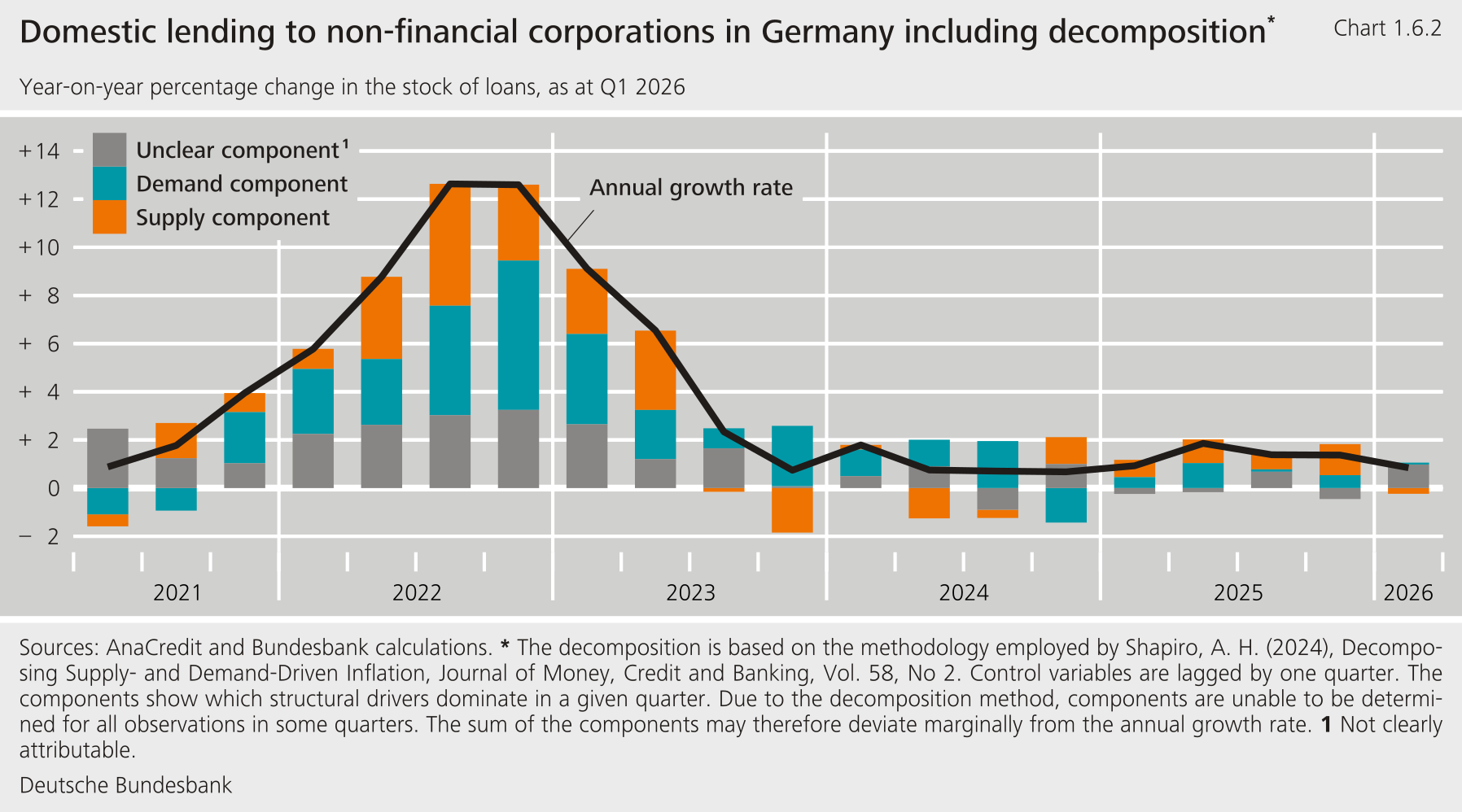
This microeconometric method enables the underlying drivers of aggregate credit dynamics to be easily identified. It is based on the bottom-up approach in Shapiro (2024) applied to granular credit data from the Analytical Credit Dataset (AnaCredit). To this end, interest rates and loan volumes are used to decompose aggregate loan growth into supply and demand components. Observations of loan growth at the disaggregated level are categorised according to whether they are predominantly dominated by supply or demand factors. Aggregating the granular observations provides insight into the relative impact of supply and demand dynamics on aggregate loan growth. 

The dataset is a panel of loan-level credit data aggregated at the banking group sector level. The dataset is based on AnaCredit data for the period from January 2020 to June 2026 and focuses on loans to non-financial corporations (NFCs) in Germany. The data are aggregated at the level of banking groups’ lending to economic sectors, resulting in 98 banking group-sector pairs (categories\(  i \) below). Aggregation at category level is necessary to avoid gaps in the data that arise due to their granular nature. The categories were left as granular as possible to maintain heterogeneity within the data. Monthly data are also aggregated on a quarterly unweighted basis. Due to the calculation of annual growth rates and the inclusion of variable lags, the estimation results are available from the second quarter of 2021.

The estimation consists of a quantity equation and a price equation that control for trends and aggregate developments. The annual growth rate of NFC loans at the category level, - Formel -, is the “quantity” and the unweighted average NFC lending rate on new loans at the category level, - Formel -, is the “price”. In the first step, two separate quantity \( (q) \) and price regressions \( (p) \) are carried out, each estimated over the entire dataset:

$$ \begin{align} q:\Delta loans_{i,t} & = \beta_0^q+\beta_1^q\Delta loans_{i,t-1}+\beta_2^q\Delta loans_{t-1}\\&+\beta_3^q\Delta interest_{i,t-1}+\beta_4^q\Delta reference rate_{i,t-1}+\epsilon_t^q \tag{1} \end{align} $$

$$ \begin{align} p:interest_{i,t} & = \beta_0^p+\beta_1^p\Delta loans_{i,t-1}+\beta_2^p\Delta loans_{t-1}\\&+\beta_3^p\Delta interest_{i,t-1}+\beta_4^p\Delta reference rate_{i,t-1}+\epsilon_t^p \tag{2} \end{align} $$

All regressors have a lag of one quarter. The regressors in both equations are the annual growth rate of NFC loans at the category level,  - Formel -, the annual aggregate growth rate of NFC loans in Germany, - Formel -, the unweighted average lending rate at category level,  - Formel -, and a maturity-adjusted reference rate based on German Federal bonds at category level, - Formel - . The error terms are  - Formel - and - Formel -.

The methodology uses sign restrictions to assign each price-quantity data point to a category that reflects the dominant structural driver. Starting from an upward sloping supply curve and a downward sloping demand curve, a shift in the axis section of the supply curve is referred to as a supply shock and a shift in the axis section of the demand curve as a demand shock. In order to apply this concept empirically, sign restrictions are used. The combination of signs of the residuals of the reduced form allows the observed innovations to be classified as positive or negative supply or demand shocks:

$$ positive demand shock: \upsilon_{i,t}^q>0, \upsilon_{i,t}^p>0→\varepsilon_{i,t}^d>0 \tag{3} $$

$$ negative demand shock: \upsilon_{i,t}^q<0, \upsilon_{i,t}^p<0→\varepsilon_{i,t}^d<0 \tag{4} $$

$$ positive supply shock: \upsilon_{i,t}^q>0, \upsilon_{i,t}^p<0→\varepsilon_{i,t}^s>0 \tag{5} $$

$$ negative supply shock: \upsilon_{i,t}^q<0, \upsilon_{i,t}^p>0→\varepsilon_{i,t}^s<0 \tag{6} $$

If the price and quantity residuals have the same sign, the observation is interpreted as demand-driven, as demand shocks move price and quantity in the same direction. By contrast, if the residuals have opposite signs, the observation is interpreted as supply-driven, as supply shocks move price and quantity in opposite directions. Observations where the residual is close to zero are referred to as “unclear”. These classifications decompose aggregate loan growth into contributions from observations dominated by demand and supply shocks:

$$ \mathbf{1}_{i\in\mathrm{demand}(+),t} = \begin{cases} 1 &\text{if } \upsilon_{i,t}^q>0, \upsilon_{i,t}^{p}> 0\\  & \text{otherwise } 0  \end{cases} \tag{7} $$

$$ \mathbf{1}_{i\in\mathrm{demand}(-),t} = \begin{cases} 1 &\text{if } \upsilon_{i,t}^q<0, \upsilon_{i,t}^{p}< 0\\  & \text{otherwise } 0  \end{cases} \tag{8}$$

$$ \mathbf{1}_{i\in\mathrm{supply}(+),t} = \begin{cases} 1 &\text{if } \upsilon_{i,t}^q>0, \upsilon_{i,t}^{p}< 0\\  & \text{otherwise } 0  \end{cases} \tag{9} $$

$$ \mathbf{1}_{i\in\mathrm{supply}(-),t} = \begin{cases} 1 &\text{if } \upsilon_{i,t}^q<0, \upsilon_{i,t}^{p}> 0\\  & \text{otherwise} 0  \end{cases} \tag{10} $$

The aggregate annual loan growth - Formel - is the sum of the loan growth of the individual categories - Formel -, weighted by their loan portfolio share from the previous year, - Formel - :

$$ \begin{align} \Delta loans_{t} = \sum_{i=1}^{n} \mathbf{1}_{i\in\mathrm{demand}(+),t} \times w_{i,t-4} \times \Delta loans_{i,t} \\+\sum_{i=1}^{n} \mathbf{1}_{i\in\mathrm{demand}(-),t} \times w_{i,t-4} \times \Delta loans_{i,t}\\+\sum_{i=1}^{n} \mathbf{1}_{i\in\mathrm{supply}(+),t} \times w_{i,t-4} \times \Delta loans_{i,t} \\+\sum_{i=1}^{n} \mathbf{1}_{i\in\mathrm{supply}(-),t} \times w_{i,t-4} \times \Delta loans_{i,t} \\+\sum_{i=1}^{n} \mathbf{1}_{i\in\mathrm{unclear},t} \times w_{i,t-4} \times \Delta loans_{i,t} \tag{11}  \end{align} $$

The approach does not reveal the relative magnitude of structural shocks and captures a wide range of price and quantity shifts. One limitation of using this approach with sign restrictions is that it can only determine whether an observation over a given period was dominated mainly by demand-driven or supply-driven contributions, but not the extent of the impact of each contribution. The decomposition should therefore be interpreted as the categorisation of components as being predominantly demand or supply driven. Further constraints on the underlying parameters would be needed to disclose the relative size of the structural shocks, but this would increase the complexity of the proposed framework. In addition, the shifts in supply and demand cover a wide range of structural shocks that move prices and quantities in a certain direction, i.e. supply shocks are at the very least a combination of monetary policy shocks and credit supply shocks.

The scenario analyses use an established model to quantify potential losses in German banks’ corporate loan portfolios. 104 It is based on granular loan-level data (AnaCredit), which contain information on the loan and the borrower. For each scenario, affected borrower groups are identified and their probabilities of default (PD) are increased according to the respective stress assumptions. Loss given default (LGD) is assumed to be constant. The resulting losses are converted into a change in the CET1 capital ratio, while risk-weighted assets are assumed to remain constant. Losses are deducted from CET1 capital. Maturing and defaulted loans are not replaced by new lending. The analyses are designed as partial stress tests, i.e. they only simulate losses in the corporate loan portfolio. Losses from other portfolios are not taken into account; the same goes for changes in risk weights or possible second-round effects caused by banks’ balance sheet adjustments. 

In the first scenario, the structural risks stress scenario, the impact of structural stress factors on credit risk in the corporate loan portfolio is analysed. Current burdens include high location costs – from high energy prices, for example – and increasing geoeconomic fragmentation. These developments weaken competitiveness, which is also under growing pressure due, in part, to the technological progress being made by Chinese enterprises. The enterprises concerned are identified in several steps. These are based on a combination of industry classification (NACE codes), input-output tables and regional characteristics.

An increase in the probability of default is assumed for enterprises that are directly affected by structural challenges. These include manufacturers, European car manufacturers and suppliers, and energy-intensive sectors of the German economy. An increase in the probability of default is also assumed for enterprises that are indirectly affected via supply chains or regional demand effects. 

Identification

Enterprises directly affected: 105

Enterprises indirectly affected via supply chains:

Enterprises indirectly affected by regional demand effects:

For all identified enterprises, the probability of default is quadrupled linearly over eight quarters and then kept constant for four further quarters. If an enterprise meets several criteria, the probability of default is nevertheless only quadrupled.

The quadrupling of the probability of default is a discretionary decision based on empirical observations in the past. The default rate for loans to the manufacturing sector in the early 2000s thus rose for German borrowers, climbing from 1.0% to 3.8% in two years. 109 In the United States, the net write-down rate for commercial and industrial loans (C&I loans) rose from 0.46% to 2.57% in the wake of the financial crisis. 110

The second scenario, the interest rate increase scenario, analyses the direct impact of a parallel rise in interest rates along the entire yield curve on credit risk in the corporate loan portfolio.

An increase in the probability of default is assumed for enterprises that could be particularly vulnerable to changes in interest rates. These include construction companies – where higher interest rates could dampen demand – developers – as project values and sales revenue could fall due to higher discount rates – and enterprises with significantly rising interest expenses due to variable rate loans or imminent refinancing.

Identification

Construction companies:

Developers:

Enterprises with significantly rising interest expenses:

For all identified enterprises, the probability of default is quadrupled linearly over eight quarters. If an enterprise meets several criteria, the probability of default is nevertheless only quadrupled.

Key restrictions

This analysis does not take into account the fact that higher interest rates may have an indirect negative impact on most firms via aggregate demand. Liabilities outside of AnaCredit are also excluded, such as loans from foreign banks or bonds that could cause further interest expenses. Moreover, the analysis ignores the fact that non-financial corporations may have hedged against interest rate increases or may benefit from higher interest income on liquid funds. For the sake of simplicity, it is also assumed that the transmission of an interest rate increase is independent of the level of the risk-free interest rate, the bank, the borrower and other characteristics.